Beam Management in a Nutshell

Beam Management in Detail

Even though 3GPP would not preclude the use of Sub 6 Ghz deployment of 5G(NR), at least based on the current status it seems that most of the deployment would be in very high frequency (millimeter wave) and this high frequency deployment would be one of the most important characteristics of 5G (NR).

• Why we need Beam ?
• Why Beam Management / Beam Control ?
• Beam Management/Control when a transmitter has no information on the location of the reciever
• Beam Management/Control when the connection is already established
• NR Beam Management in a Nutshell
• Where to point my beam ?
• When receiving
• When transmitting
• How can UE detect / aquire a beam for initial attach ?
• P1, P2, P3 - What is It ?
• How Beam Switching happens ?
• Building Up Intuition
• How is a beam formed ?
• How the shape of the beam changes with the number of antenna ?
• How to change the direction of beam (beam steering) ?
• How the shape of steering beam changes with the number of antenna ?
• How the distance between antenna elements affects the shape of radiation pattern ?
• How to interpret the CSI Codebook table intuitively ?
• From Intuition to 3GPP

Why we need Beam ?

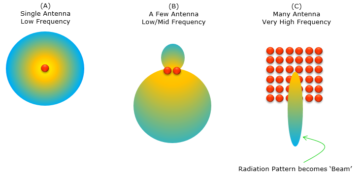
Mostly by Nature of the wave (by Physics), when we use low and mid range of frequency, we can transmit a signal in all direction (as in (A)) or relatively wide angles (as in (B)). However, when we use very high frequency, we would not have much choice except using a huge antenna array. As a result of using this kind of huge antenna array, the resulting radiation would be a beam as in (C). Refer to Why Massive MIMO page for the details of this background.

Why Beam Management / Beam Control ?

I don't think trasmitting signal in Beam in high frequency deployment would be the matter of choice. It is a kind of 'MUST' implementation. In case of low / mid frequency region without using massive antenna array (as in (A) / (B)), a single transmission would cover a lot of UEs simultaneously. However, when the radiation become beam-shaped as (C), it is very difficult to cover multiple UEs in single transmission unless those multiple UEs are located in very close proximity. To handle this problem, we need a very sophisticated idea of managing/controlling the beam to cover the multiple devices scattered in all directions and the management/control mechanism should be different depending on the situtations. All of these collection of idea would fall into the title of "Beam Management" in the specification.

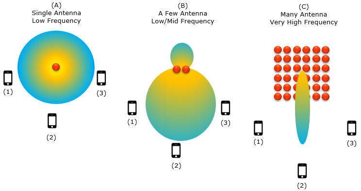
Beam Management/Control for each specific situation will be described in separate pages with relavent situation (like Beam Management during Synchronization, Beam Management during Initial Attach, Beam Management in connected status etc). In thise page, I would describe on general idea.

Beam Management/Control when a transmitter has no information on the location of the reciever

Now let's look into a more specific cases where the Beam Management/Control become crucial. As an example, let's think of following case. There is a Base Station with Massive MIMO operating at the very high frequency. There is a UE around the Base Station and you are just about to turning on the UE. Once the UE is turned on, it would start Synchronization process. For this step, the Base Station would transmit the special signal called Synchronization Signal and the signal should be able to reach to every UEs around the base station. However, here comes a serious problem with the base station sending signal in Beam. It is the fact that the signal beam can point to a very narrow area and it cannot cover a very wide area at the same time. Simply put, now you have the following question.

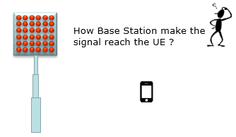
What would be the answer for this ? If everything works as you draw in power point, you may draw a solution as follows. You may want to transmit a lot of beams in all direction simultaneously. Looks good ? Looks like a flower :).

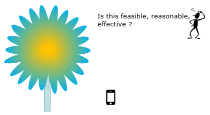
Would the solution above be feasible, reasonable and effective ? The simple answer is NO (I would not explain why. You may easily guess why).

Then what can be another idea (possible soultion) for the problem ? There can be multiple ideas and proposals, but the most popular proposal as of now seems to be that the base station transmit the beam to a specific direction at a specific time and then change the direction a little bit in a next time frame and so on until it can scan all the area it should cover.

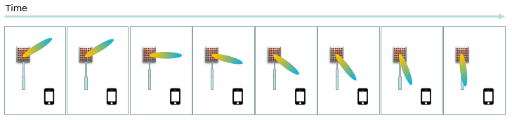
Then, the next question would be "how to reflect / implement this concept in the radio frame design ?". I would not go too much detail on this until this is explicitely determined in 3GPP TS (Technical Specification) document, but you can get the general ideas on various options /proposals from TDocs listed in Reference Section.

// Now that 3GPP Technical Specification on Beam Management has been released and I could write on this mechanism based on the formal specification. You may jump to NR Beam Management in a Nutshell section and read from there if you are interested in the formal specification.

Beam Management/Control when the connection is already established

Now let's talk about more serious case of Beam Management. In terms of 3GPP TDocs, Beam Management handles mostly with this topic (Beam Management during the connected states) and the one mentioned in previous section are described as a part of the topic Cell Search / Initial Access.

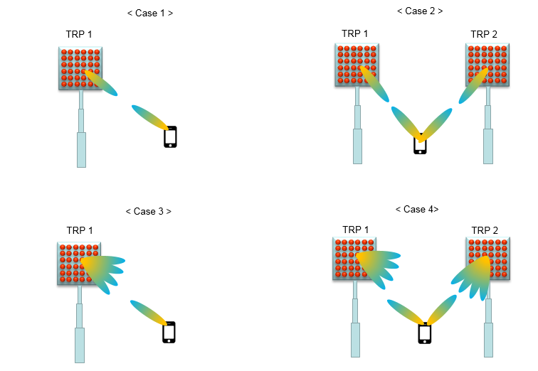
Once UE gets into a connection states with a Network, at least one beam (or multiple beam) is properly in connection between UE and the network. Theretically there can be so many different ways in which UE and Network beam is connected, but we can reduce it down to roughly four differences case as shown below.

In case 1, UE and Network is connected through a single TRP (Tx/Rx Point) and a single beam.

In case 2, UE and Network is connected through multiple TRP (Tx/Rx Point) and a single beam for each TRP.

In case 3, UE and Network is connected through a single TRP (Tx/Rx Point) and multiple beams

In case 4, UE and Network is connected through multipe TRP (Tx/Rx Point) and multiple beams for each TRP

You may think of many other cases and ask "How about this case ? How about that case ?". Whatever you think of and whatever you are asking, I think all of those would be valid thinking and valid question until 3GPP reach a explicit conclusion. So keep asking and try to find your own answers until you see the explicit 3GPP specification.

Now the important and tough task is to maintain the connection. For this, I would not write much details until 3GPP specifies it in detail. Sorry for skipping too much with the execuse of 3GPP specification unavailability :). But I don't want to write many things now and rewrite too much after 3GPP Technical Specification come out. For now, my purpose is to give you very broad and general idea, and let you know what you may need to study in further details if you are really interested in technical details. For this purpose, I will list up most of TDocs about each topics in Reference section, so that you can get more detailed idea proposed by many companies / organizations in the industry.

The general idea of the beam management during the connected states would be

i) Network transmit a specific reference signal for beam management

ii) UE detect the signal and perform some measurement and send feedback to Network

As you may notice, the general idea would be very similar to CSI report mechanism that are currently used in current LTE. However, a lot of details are yet to be determined.  For example,

i) Baseband Signal (Symbol) generation formula

ii) Resource Allocation mapping (How to allocate these reference symbols to which specific resource element)

iii) How often UE need to perform these measurement

iv) How UE report the measurement result ? (via RRC messages ? or via MAC / PHY layer transactions ?)

NOTE : Now that the technical specification on all of the questions listed above has been released and I wrote a few separate pages regarding this topic. Refer to CSI RS signal page and CSI Report page for further details based on 3GPP technical specification.

NR Beam Management in a Nutshell

If you ask me to explain about NR Beam Management in a few seconds, I would summarize the whole process in an illustration as shown below. As you see here, Beam Management plays important role in two period - During RACH procedure and After the call connection.

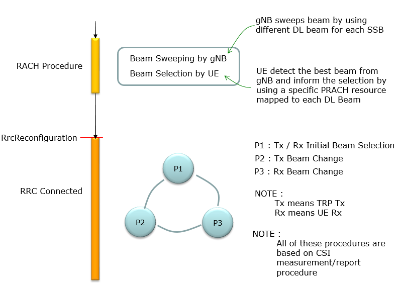
Let me walk through that illustration piece by piece, because it packs most of this page into one picture. There are three parts to it. The vertical bar on the left is time. The box at the top right is what happens during RACH. The ring of three circles at the bottom right is what happens once the UE is connected.

Look first at where the two phases meet. The boundary is not labelled 'connection'. It is labelled RrcReconfiguration, and that is a deliberate detail. Before that message arrives, the only downlink beams the UE can measure are the SSB beams, and those are broadcast to the whole cell. After it, the UE has its own CSI-RS resources and its own report configuration. So that line marks the moment beam management stops being common to everybody and becomes specific to one UE. Everything drawn below the line is possible only because that configuration now exists.

The upper half has just two roles, and the picture names them both. First, gNB sweeps its beams, using a different downlink beam for each SSB. Then UE detects the best one and informs gNB of its choice. The interesting part is how that choice travels. The annotation says it plainly : the UE uses a specific PRACH resource mapped to each downlink beam. There is no message carrying a beam index, because at that point there is no channel to carry one. This is the mechanism described in the initial attach section further down this page.

Now look at the bottom half, and notice that it is drawn as a ring rather than an arrow. That is not just decoration. P1, P2 and P3 are not a sequence that runs once and then stops. They keep cycling for as long as the connection lasts, because the UE keeps moving and the channel keeps changing.

The legend beside the ring is worth reading slowly. P1 is initial beam selection, for Tx and Rx together. P2 is a Tx beam change. P3 is an Rx beam change. Then comes the note that saves a lot of confusion : Tx here means the TRP transmit beam, and Rx means the UE receive beam. So P2 changes what gNB is doing, and P3 changes what the UE is doing. One more word deserves care. The 'initial' in P1 means initial within connected mode. It has nothing to do with initial access.

The second note under the ring is the one that carries the most weight. All three procedures rest on the CSI measurement and report procedure. That is the machinery that lets the UE tell gNB what it is seeing. Without it, nothing in the lower half of the picture would work at all. It is also why that topic ends up needing a page of its own.

If you would rather have the same picture as a map of the rest of this page :

Read down the third column and the whole story shows up in one move. Before a connection exists, the UE can only answer by choosing a resource. Once the connection exists, it can answer with an actual report. And if the serving beam collapses, it falls straight back to choosing a resource again. Beam failure recovery is, in that sense, the picture folding back to its own top half.

Where to point my beam ?

This question sounds trivial, but it has no default answer. With a wide beam you never have to ask it. The energy goes more or less everywhere, so the receiver ends up inside the coverage whatever it does. A narrow beam takes that comfort away. The energy now travels in one direction only. If the two ends disagree about which direction that is, there is no link at all. Both radios can be working perfectly and you would still see nothing.

It is also four questions rather than one. Each end of the link has to point twice, once for transmitting and once for receiving. On the network side, gNB has to decide where to aim its downlink, and where to listen for the uplink. On the device side, UE faces exactly the same two decisions in the opposite direction. So a single connection needs four pointing decisions to line up at the same time.

Then why split them into 'transmitting' and 'receiving' rather than into 'gNB' and 'UE' ? The reason is that the logic follows the role, not the box. A transmitter always has the same problem. It has to commit to a direction before it sends anything. A receiver always has the same problem too. It has to be tuned already before the signal arrives. Whether the box is a base station or a handset changes the details. It does not change the shape of the question.

That word 'before' is where the difficulty lives. You cannot measure a signal you have not sent yet, and you cannot measure one that has not arrived yet. So every answer in the next two sections is really an answer about the past. Both ends point on the basis of something they measured earlier, and then trust that the channel has not changed much since. This is also the reason why beam management never stops while the connection is up.

One more idea makes all of this a lot cheaper, and it is worth naming before you meet it below. If a device knows the best direction to receive from, it can often assume that the same direction is the best one to transmit to. This assumption is called beam correspondence. When it holds, a single measurement answers two of the four questions at once. When it does not hold, the transmit direction has to be found separately, and that costs extra signalling.

We can think of this question in terms of two different cases : transmitting case and receiving case.

When transmitting,

Now let's think of which direction a gNB or UE has to point its beam when they try to transmit the signal ?

The answer is simple.  They (gNB or UE) has to transmit the signal in the direction that can reach the reciever with the best signal quality.

Then you would have another question. How can they(gNB or UE) figure out which direction is the one that can reach the reciever with the best signal quality ?

Now the answer would be a little bit trickier, but the big picture is as follows.

• When gNB is transmitting, gNB figure out this direction by evaluating the quality of a specific reference signal of multiple beam from UE. gNB evaluate the quality of the reference signal from each of the multiple beam and chose the best one. The reference signal from UE is called SRS.
• When UE is transmitting, UE figure out this direction by evaluating the quality of a specific reference signal of multiple beam from gNB. UE evaluate the quality of the reference signal from each of the multiple beam and chose the best one. The reference signal from gNB in this case can vary depending on situation. Sometimes it can be SSB and sometimes it can be CSI-RS. (NOTE : CSI-RS play many different roles in addition to beam management and very complex topic. Refer to CSI-RS signal generation and CSI report page for further details).

NOTE : This kind of estimation of reference signal quality should be done sometime before they transmit signal.

3GPP TR 38.802 (V14.2.0)-6.1.6.1 describes on this situation as follows :

• TRP is able to determine a TRP Tx beam for the downlink transmission based on TRPs uplink measurement on TRPs one or more Rx beams
• UE is able to determine a UE Tx beam for the uplink transmission based on UEs downlink measurement on UEs one or more Rx beams

NOTE : TRP is a transmission point of a gNB.

Notice what all of those statements have in common. In every one of them, the transmitter picks its direction from something it received earlier. Nothing is measured about the transmission itself. That is the shortcut named at the start of this section. On the UE side it is called beam correspondence, and on the gNB side it is ordinary channel reciprocity. NR in FR2 is TDD, so uplink and downlink sit on the same frequency, and the assumption is a reasonable place to start.

It is still only an assumption though, and it is worth knowing where it breaks. Beam correspondence is a UE capability, not a law of physics. Separate transmit and receive hardware paths, imperfect antenna calibration and strong interference can all pull the best transmit direction away from the best receive direction. 3GPP therefore defines beam correspondence requirements that a UE has to meet. A UE that cannot meet them has to find its uplink beam the slow way, by sweeping. That sweep uses an SRS resource set with its usage set to 'beamManagement'.

There is also a second route for the downlink, and in FR2 it is the one you will meet most often. Rather than deriving its transmit beam from SRS, gNB can simply ask. UE measures the candidate beams, reports the best one back, and gNB transmits on that beam from then on. This is exactly what P1 and P2 do, and they are described later on this page. Both routes are real, and a live network normally uses both. The reporting route needs no reciprocity assumption at all, so it keeps working even when beam correspondence does not.

Putting the two routes side by side :

NOTE : The last row is the fallback for a UE without beam correspondence. In that case gNB measures the UE uplink beams itself. It then tells the UE which one to use, through an SRI field or a spatial relation. See How Beam Switching happens for how that indication is carried.

When recieving,

Now let's think of which direction a gNB or UE has to point its beam when they try to recieve signal ? (In this case, the word 'beam' may be a little misleading because the reciever does not form any real beam. So it would be better to change the phrase 'to point its beam' to 'to tune its reciever to a certain direction').

The answer is simple.  They (gNB or UE) has to tune their reciever in the direction in which they can receive the signal from the transmitter with best quality.

Then you would have another question. How can they(gNB or UE) figure out which direction is the one in which they can receive the signal from the transmitter with best quality ?

Overall logic is as follows :

• When gNB receiving signal from UE, (before doing this) gNB is supposed to get the information of the best direction from UE in the form of CSI report.
• When UE receiving signal from gNB, (before doing this) UE is supposed to get the information of the best direction from gNB (gNB has detected the best direction based on the measurement of SRS signal quality of multiple beams from UE and indicates the UE of the best direction).

3GPP TR 38.802 (V14.2.0)-6.1.6.1 describes on this situation as follows :

• TRP is able to determine a TRP Rx beam for the uplink reception based on UEs downlink measurement on TRPs one or more Tx beams.
• UE is able to determine a UE Rx beam for the downlink reception based on TRPs indication based on uplink measurement on UEs one or more Tx beams.

There is one more thing worth pulling apart here, because it is a common source of confusion. Choosing a receive direction is really two decisions rather than one. The first is 'which transmit beam should I be expecting ?'. The second is 'which of my own receive beams works best for that one ?'. The two are answered by different parties, and at different speeds.

For the UE, the network answers the first question. It does that by telling the UE which reference signal the incoming transmission is spatially related to. That pointer is carried in a TCI state, and it is the mechanism described in How Beam Switching happens. Without it, the UE would have no way of knowing which of the many beams around it is the one meant for it.

The UE answers the second question on its own. In P3, gNB repeats the same transmit beam several times in a row. The UE tries a different receive beam on each repetition and keeps whichever one worked best. One detail here surprises people the first time : the UE never reports the answer. The result stays inside the UE, because gNB does not need to know which receive beam won. It only needs to know that the UE can hear the beam it is sending.

The same split exists on the gNB side, with the roles swapped. To choose its own receive beam, gNB measures SRS from the UE across its candidate receive beams and keeps the best one. Alternatively it can simply reuse the beam it already found for the downlink, and that is the reciprocity route quoted just above.

So the four pointing decisions raised at the start of this section are answered like this :

Look down that table and one pattern stands out. The two transmit decisions leave a trace in the signalling, either as a beam report or as an SRI. The two receive decisions leave nothing behind. Each receiver picks its own beam privately, and the other end never learns which one it settled on. This is why receive beam problems are so much harder to chase down in a log than transmit beam problems.

How UE detect / aquire a beam for initial attach ?

Everything up to this point quietly assumed that a connection already exists. The network knows the UE is there, and the UE knows where the network is. The two can then exchange measurements and refine what they know. Initial attach has none of that. The UE has just been switched on. The network has no idea that it exists. So neither side can point at the other, and neither side can ask.

This is a real chicken and egg problem, and it is worth staring at for a moment. The answer used in connected mode was 'point on the basis of something you measured earlier'. At initial attach there is nothing measured earlier. There is also nothing to report it with. The UE has no uplink grant, no identity in the cell, and no channel to carry a measurement. So whatever mechanism we use has to work with zero prior knowledge and zero uplink signalling.

The network half of the problem was already described in an earlier section. The reason gNB sweeps at all is that it cannot usefully transmit in every direction at once. So it transmits in one direction at a time and cycles through them. Each of those transmissions is an SSB, and every SSB carries its own index. That index is what makes one beam distinguishable from another. FR1 uses up to 4 or 8 of them depending on the band, and FR2 uses up to 64. The whole burst fits inside a 5 ms window, and during initial access the UE assumes it repeats every 20 ms.

Now comes the part that I find genuinely clever. The UE picks the strongest SSB, and then it has to tell gNB which one it picked. But it has no message to put that in. There is no RRC connection yet, and no uplink grant either. So the answer is not carried in the content of a message at all. It is carried in the choice of resource. Every SSB index is mapped to a particular set of PRACH occasions and preambles, and that mapping is broadcast in SIB1. When the UE transmits PRACH on one of those resources, the resource itself says which beam it heard.

That one trick is what gets the whole process off the ground. Once PRACH arrives, gNB looks at which resource it landed on. It now knows roughly which direction the UE is in. So it can send the random access response on that same beam, rather than sweeping blindly all over again. From that point on the UE is reachable and a feedback channel finally exists. The P1, P2 and P3 processes described later can then take over the job of refining the beam.

Simply put, gNB transmit a sequence of SSB beam with different direction and UE detect the best beam among them and send PRACH to the location which is mapped to a specific SSB beam ID (i.e, gNB figure out the SSB beam that a UE detected by the PRACH location it received from the UE). For further details, see this note. For animated version of this process, check out my visual note here.

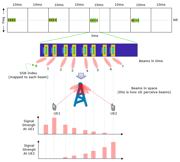
Let's take a little bit deep dive into this case and describe each part of the illustration verbally.

• i) gNB is transmitting 8 consecute SSB with same power in beam directing in different directions.
• ii) Following happens on UE1
• UE1 does not trigger PRACH as soon as it detect a SSB. It tries to detact all the SSB configured in RRC.
• UE1 detected 7 SSBs out of the 8 SSBs transmitted by gNB. Even thought gNB transmits all the SSBs in same power
• UE1 percieves each of the beam power differently because alignment of UE antenna and the direction of each SSB beam varies.
• UE1 compares the received SSB power and pick the best SSB (SSB 1(the second SSB) in this case).
• UE1 transmit PRACH using the physical resources mapped to SSB 1
• iii) Following happens on UE2

• UE2 does not trigger PRACH as soon as it detect a SSB. It tries to detact all the SSB configured in RRC.

• UE2 detected 6 SSBs out of the 8 SSBs transmitted by gNB. Even thought gNB transmits all the SSBs in same power

• UE2 percieves each of the beam power differently because alignment of UE antenna and the direction of each SSB beam varies.

• UE2 compares the received SSB power and pick the best SSB (SSB 7(the eight SSB) in this case).

• UE2 transmit PRACH using the physical resources mapped to SSB 7

P1, P2, P3 - What is It ?

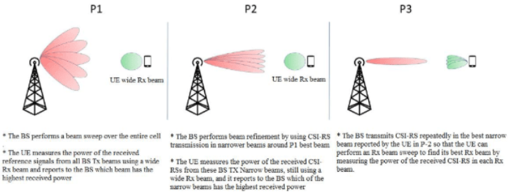
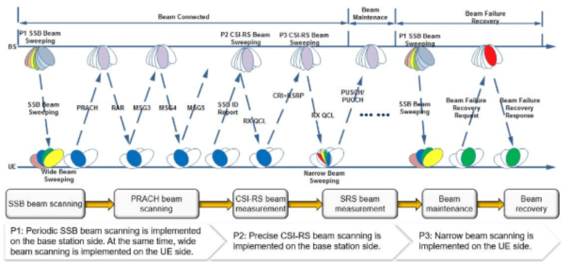
As illustrated in Beam Management in a Nutshell, P1/P2/P3 are a set of processes that are designed for beam management while in connected state.

I will talk about a high level view on these processes in this section. For further details, you would need to understand the very details on CSI report for Beam Management which is another huge topic and will be described in a separate page here.

Before going into what each of them does, it is worth asking why there are three of them at all. Why not a single procedure that just finds the best beam and be done with it ? The reason is that 'the best beam' is not one unknown. It is three. The first is which gNB beam is roughly the right one. The second is which narrower gNB beam is best inside that rough area. The third is which of the UE own receive beams works best against it.

There is a very practical reason behind the split as well, and it is really a counting argument. Suppose gNB has 64 beams to choose from and the UE has 8. Trying every combination means 64 times 8, which is 512 pairs. Sweeping 512 pairs every time the user turns their hand is not affordable. Staging the search changes that arithmetic. Instead of multiplying the two searches together, you add them. This is the real reason the procedure is staged rather than exhaustive.

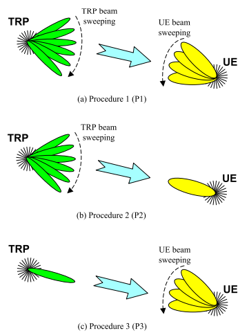
Once you look at it that way, the pattern behind P1, P2 and P3 becomes easy to remember. In every stage, one side holds still while the other side searches. P1 is the coarse stage that finds a working pair starting from nothing. P2 holds the UE receive beam still and refines the gNB transmit beam. P3 holds the gNB transmit beam still and refines the UE receive beam. A search only makes sense if the other end is not moving at the same time.

One practical warning before you go hunting for these names in the specification. You will not find them there. P1, P2 and P3 come from the study phase, and the formal wording quoted later in this section is from TR 38.802. The industry kept the names, but the technical specifications never use them. What you actually configure is a CSI-RS resource set with a parameter called repetition. When repetition is off, the UE cannot assume the resources share a transmit beam, so gNB is sweeping and the UE holds still. That covers P1 and P2. When repetition is on, the UE may assume every resource uses the same transmit beam, so the UE is free to sweep its own. That is P3, and its report quantity is typically none, because there is nothing for the UE to tell gNB.

One last thing worth keeping in mind. P1, P2 and P3 are not a sequence that runs once and then finishes. P1 keeps running quietly in the background, and P2 and P3 get triggered again whenever the link starts to degrade.

In short, P1,P2,P3 is all related to downlink beam management. that is, it is a mechanism for UE to better receive the downlink beam(data). There is another mechanism for uplink beam management(i.e, U1, U2, U3).. but this is not strictly formalized in 3GPP specification. The functionality of P1,P2,P3 can be summarized as follows.

More formal definition of these process are stated in 38.802-6.1.6.1, P1/P2/P3 as follows.

P-1: is used to enable UE measurement on different TRP Tx beams to support selection of TRP Tx beams/UE Rx beam(s). For beamforming at TRP, it typically includes a intra/inter-TRP Tx beam sweep from a set of different beams. For beamforming at UE, it typically includes a UE Rx beam sweep from a set of different beams.

Does this make sense to you ? It may take time to get clear understanding on this. Following illustration is my understanding/interpretation of this statement. (Click on the image to see the animated/slide show version)

P-2: is used to enable UE measurement on different TRP Tx beams to possibly change inter/intra-TRP Tx beam(s). From a possibly smaller set of beams for beam refinement than in P-1. Note that P-2 can be a special case of P-1.

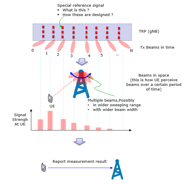
Following is my understanding on this process in illustration. (Click on the image to see the animated/slide show version)

P-3: is used to enable UE measurement on the same TRP Tx beam to change UE Rx beam in the case UE uses beamforming

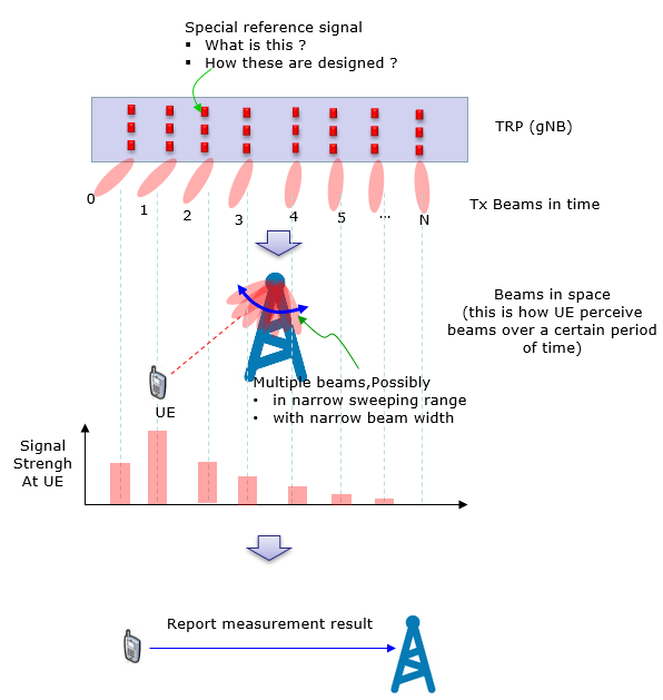
Following is my understanding on this process in illustration.

NOTE 1 : I put a visual note here to give some intuitive understandings on this process. This visual note may apply to P1, P2 (not P3)

NOTE 2 : I think the beam management procedure may be confusing at the early stage of the study. My personal way to tackle those confusing concepts when I am learning a new technology is to check with the explanation for the same concept from various other sources. Those different sources would share large portions of commonalities but each of the sources would present a little bit different aspect of the same concept. As you go through those materials from various other sources, your brain would automatically consolidate all those diverse representation and come up with some new presentation of your own.  I wish I can get everybody to understand everything from my note only :), but I know it is not possible.

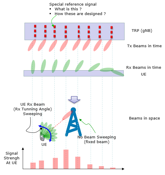
Just to help you with searching different sources, I would add presentations from a few different sources from here.

I found a little bit of simplified illustration of P1, P2, P3 process from this paper ([17]) as shown below :

Following illustration is from a document from 5gworldpro.com with approval to share it in this note. 5gworldpro.com provides various types of 5G related training as well.

How Beam Switching happens ?

P1, P2, P3 in the previous section answers the question 'which beam is the best one ?'. But knowing the best beam and actually using it are two different things. Somewhere between the measurement and the data, a decision has to be made. Then both sides have to start using the new beam at exactly the same moment. That part is what I call Beam Switching here. It is the dynamic beam change that keeps happening while the UE stays in connected mode.

Why does this need a mechanism of its own ? Just think of what would happen if the UE changed its receive beam whenever it felt like it. gNB would still be transmitting in the old direction and UE would be listening in the new direction. The link would simply die. So a beam change has to be commanded by the network, and it has to happen at a timing that both sides can calculate. This is the reason why 3GPP spends so much signalling on an operation that sounds so simple.

First of all, how is a beam represented in signalling ?

This is the part that confuses most people at the beginning (it confused me for quite a long time). gNB never tells the UE 'turn your beam 30 degrees to the left'. gNB has no idea where the UE antenna is pointing, and it does not need to know. What gNB actually says is something like 'receive this channel with the same spatial filter that you used when you received SSB #3'.

This 'use the same spatial setting as that reference signal' is exactly what QCL (Quasi Co-Location) means. The QCL type that carries the beam information is QCL-TypeD (Spatial Rx parameter). The container that holds this pointer is called a TCI state (Transmission Configuration Indication state). So in NR signalling, the mapping goes like this :

• a beam becomes a TCI state
• a TCI state is a pointer to a reference signal (SSB or CSI-RS) plus the QCL type
• changing a beam becomes changing the TCI state

If QCL is a new concept to you, I would read this note first. Without QCL, the rest of this section would not make much sense.

Three layers : RRC, MAC CE and DCI

NR does not use a single message to change a beam. It uses three layers and each of them runs at a different speed.

Why bother with three layers instead of one ? It is a trade between how fast you can signal and how much you can say. RRC can describe everything but it is slow and it costs a reconfiguration. DCI arrives every slot but it only has 3 bits, which is 8 values, and 8 values cannot address 128 configured states. MAC CE sits in the middle and solves exactly this. It narrows 128 candidates down to the 8 that matter right now, so that the 3 bit DCI field becomes enough. Once you see this, the whole beam signalling design suddenly looks reasonable rather than complicated.

PDCCH and PDSCH do not switch the same way

This is a detail that trips up a lot of people reading a log for the first time. The two downlink channels are switched by different mechanisms.

PDCCH beam is tied to the CORESET, not to a single transmission. Each CORESET has one active TCI state, and it is changed by a MAC CE (the TCI State Indication for UE-specific PDCCH MAC CE). There is no per-slot beam switching for PDCCH. That makes sense, because the UE has to know where to look before it can decode anything at all. Details of that MAC CE are in this note.

PDSCH beam can change per scheduling. The DCI (format 1_1 or 1_2) carries a 3 bit Transmission Configuration Indication field. The codepoint to TCI state mapping itself comes from a MAC CE. See this note for that one. However, this field exists only when tci-PresentInDCI is enabled for the CORESET. If it is not enabled, PDSCH simply follows the beam of the CORESET that scheduled it.

The timing : when exactly does the new beam start ?

This is the part that really matters in practice, because gNB and UE must switch together. There are two different rules and they apply to the two different mechanisms.

Take the MAC CE based switch first. The new TCI state applies from 3 ms after the HARQ-ACK for the PDSCH that carried the MAC CE. The exact wording in the specification counts slots rather than milliseconds, but 3 ms is the number worth remembering. Note that the reference point is the ACK, and not the moment the MAC CE was received. This is deliberate, because gNB only knows that the UE really got the command once the ACK comes back.

For a DCI based switch, the constraint is a UE capability called timeDurationForQCL. It is the time the UE needs between decoding the DCI and being ready to receive with the new beam, expressed in symbols. If the gap between the DCI and the scheduled PDSCH is larger than this value, the UE applies the TCI state that the DCI indicated. If the gap is smaller, the UE has no time to retune, so it falls back to a default beam instead. In Rel-15 that default is the TCI state of the CORESET with the lowest ID in the latest monitored slot.

NOTE : That fallback rule is worth keeping in mind when you see a beam that does not match what the DCI asked for. It is not always a bug. Very often it just means the scheduling offset was shorter than timeDurationForQCL.

Uplink beam switching

Everything above is about the downlink. The uplink has its own set of handles. The table below collects all of them in one place, so that you can see the pattern.

Notice the indirection in the PUSCH row. The DCI does not name a beam. It names an SRS resource, and the beam is whatever that SRS resource was configured to use. This is the uplink version of the same idea as QCL. A beam is always identified by pointing at another signal, never by an angle.

Rel-17 : the unified TCI framework

Did the previous two sections feel like a lot of separate mechanisms for one simple idea ? You are not the only one. Rel-15 ended up with a different beam handle for almost every channel, and each of them had to be updated separately. In a FR2 cell where the UE is moving, that is a lot of signalling just to keep pointing at the same place.

Rel-17 introduced the unified TCI framework to fix this. The idea is that one beam indication applies to all, or at least most, of the channels at once. It comes in two flavours. A joint TCI state covers downlink and uplink together, which is the natural choice when beam correspondence holds. Separate DL and UL TCI states are used when the two directions need different beams. The indication itself is carried in DCI format 1_1 or 1_2, and it may come either with or without an actual downlink assignment. That second option is useful, because it means gNB can update the beam without having to schedule data just to carry the indication.

What if the switch does not make it in time ?

Beam switching as described here is the well behaved case, where the network still has a working beam to send the indication on. In FR2 that assumption breaks more often than you would like. A hand, a body or a passing vehicle can drop the serving beam in an instant. That is far faster than a measurement report and a MAC CE can travel. When that happens, the UE is left listening on a beam that no longer works, and the network cannot reach it to fix the problem.

That is exactly what Beam Failure Detection and Beam Failure Recovery are designed for. The topic deserves its own note rather than a paragraph here. See this page for the details.

One more case worth knowing about is when the better beam belongs to a different cell rather than a different direction of the same cell. Up to Rel-16 that meant a normal handover, with all of its RRC signalling and interruption. Rel-18 added L1/L2 triggered mobility (LTM), which makes the cell change look much more like the beam switch described in this section. Refer to this note if you are interested.

Putting it together

• A beam is never signalled as a direction. It is signalled as a pointer to a reference signal, wrapped in a TCI state, and QCL-TypeD is the part that carries the spatial meaning.
• RRC configures the pool, MAC CE activates a working subset, DCI picks one of them. The three layers exist because 3 bits cannot address 128 states.
• PDCCH switches by MAC CE only, and PDSCH can switch per scheduling. The UE has to know where to look before it can decode anything, so the control channel gets the slower and safer mechanism.
• Timing is not a detail here, it is the whole point. MAC CE based switching applies 3 ms after the HARQ-ACK, and DCI based switching needs the scheduling offset to be at least timeDurationForQCL.
• If the scheduling offset is too short, the UE uses a default beam instead of the indicated one. A beam that does not match the DCI is often this rule, and not an error.
• Uplink uses the same pointing idea under different names. PUCCH and SRS use a spatial relation. PUSCH uses an SRI that points at an SRS resource.
• Rel-17 unified TCI collapses all of these into one indication, and Rel-18 LTM extends the same style of fast switching across cells.

Building Up Intuition

Usually when a designer/inventor postulate any technology or theory, they first come up with those idea in their brain in intuitive way and then formulate those idea in various formal documents like technical papers, thesis or industry document. These formal document would be easily understood by those who has similar level of experties as the original designer, but for those who does not have the same level of experties or experience, it is very hard to get the clear picture just by reading the formal documents. I think the best way to build up intuition is to try things with your own hands and see the result with your own eyes, but it is not always easy to have this kind of physical setups especially for Beam related issues. Then, what would be the alternative to the physical setup ? My alternative is to use software simulator like Matlab. Actually this kind of software simulator give some additional advantage.

• You can try many things with easy and in very short time (almost no preparation / setup time).
• You can visualize many things that cannot easily be done by physical setup (like visuallizing beams).

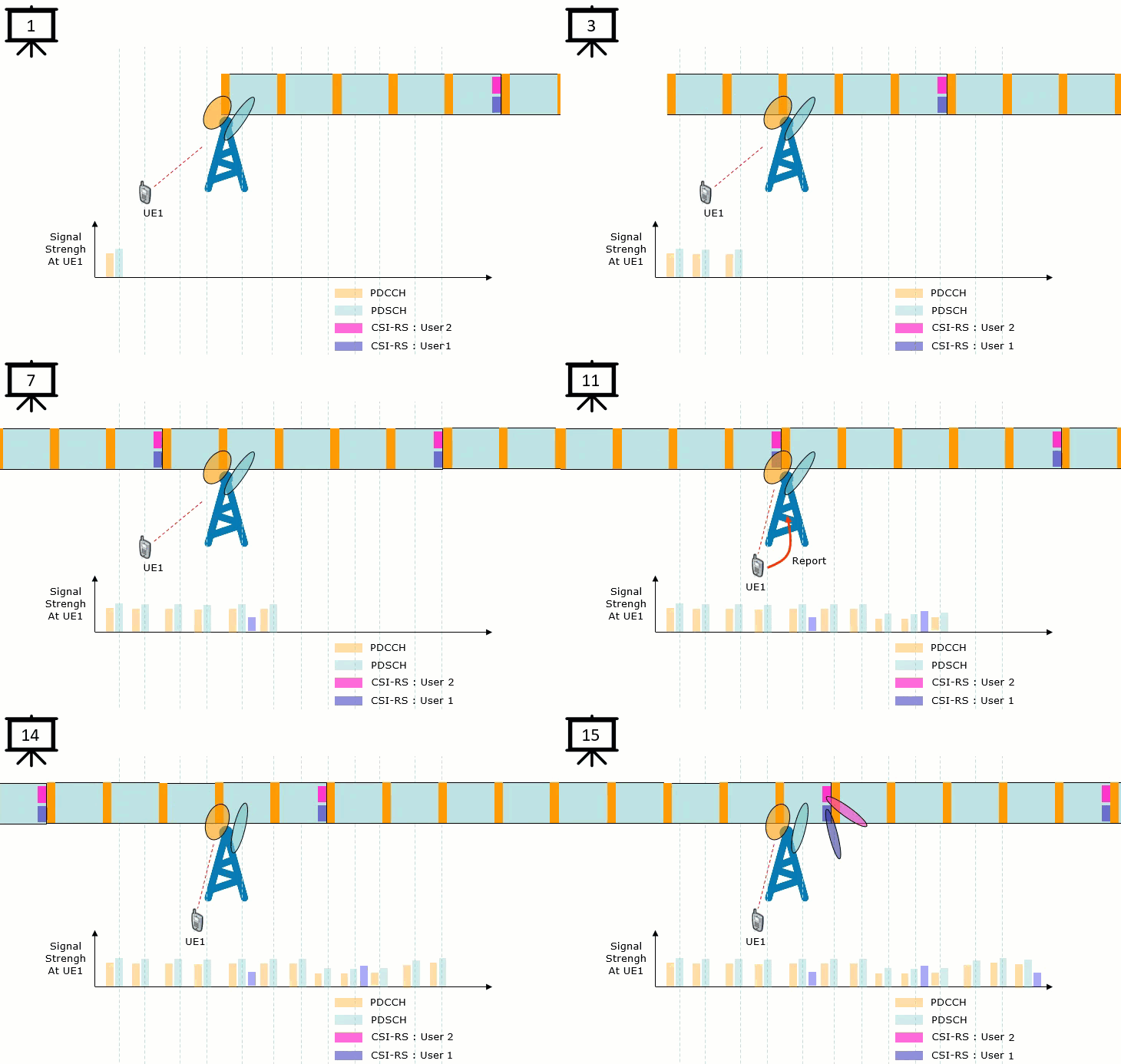
Before you are trying to build any intuition, it would be very helpful if you have some questions in your mind and trying to come up with some intuitive answer to the questions. Following is some questions of my version.  Below the question are the links to other pages in which I wanted to try to answer it in my way (intuitive way). If you follow the link, you would see several buttons as shown below. You can move forward/backward, animate forward/backward the sequence of images. Most of these pages are from another type of my note here.

How is a beam formed  ?

The short answer is that a beam is not something an antenna pushes out in a direction. It is what is left over after a lot of waves cancel each other everywhere else. That reversal is the whole idea, and it is worth getting straight before anything else. A single element radiates over a very wide angle, and nothing you do to that one element will change it. What you can do is put several elements next to each other and let their waves interfere.

This is exactly why the water ripple picture works so well as a starting point. Drop two stones into still water at the same moment. Each one sends out its own circular ripple. Where two crests meet, the water rises higher than either ripple alone. Where a crest meets a trough, the surface stays flat. What you end up with is a fixed pattern of strong lines and dead lines, spreading outward from the pair of stones. Nobody aimed anything. The pattern is simply where the arithmetic came out positive.

That is exactly what the picture below shows. In the left panel there are 8 pebbles, evenly spaced, all dropped at the same instant. The middle panel catches the moment each one starts its own circular ripple. In the right panel the ripples have met each other, and the orange ellipses mark where the crests keep reinforcing.

Two things in that last panel are worth pausing on. The strong directions come out perpendicular to the line of pebbles, straight up and straight down. And between them the water is almost flat, even though every pebble is still sending waves that way. That flat region is the cancellation doing its work. Because all 8 pebbles were dropped at the same instant, the pattern is symmetric and points straight ahead. This is the broadside case, and the steering section further down is what happens when you stop dropping them at the same instant.

So what decides whether a particular direction gets a crest or a trough ? It is the difference in distance from each element to that direction. Look at the array from straight ahead and every element is the same distance from you. Look at it from an angle and each element sits a little further away than the one before it. If the spacing is d and the angle away from straight ahead is theta, that extra distance works out as d times sin(theta) per element.

Distance then turns into phase, by comparing it with the wavelength. An extra path of one whole wavelength puts the wave back exactly in step, so the contributions add up. An extra path of half a wavelength puts it exactly out of step, so they cancel. Every angle in between lands somewhere between those two extremes. The radiation pattern you see plotted is nothing more than that calculation repeated for every direction.

Two consequences fall out of this, and they happen to be the next two questions on this page. Adding more elements makes the cancellation sharper, so the beam gets narrower. And if you deliberately delay each element by a fixed amount, you move the direction in which everything adds up. That is beam steering, and notice that neither of them requires the antenna to physically move.

The animation below is the two stone version of this. It is worth watching the pattern build up rather than just looking at the final picture.

• Interference of Water Ripple

How the shape of the beam changes with the number of antenna ?

The previous question showed that a beam is an interference pattern. This one asks what happens when you add more sources to that pattern. The short answer is that the beam gets narrower and stronger, and it does both at a rate you can work out in advance.

Think again about where the cancellation comes from. With two elements there are only two waves available to cancel each other, so the cancellation is never very thorough. Move a little off the main direction and the two are still roughly in step. With sixteen elements there are sixteen waves, and they only all line up over a very narrow range of angles. Step slightly off that direction and the sixteen phases fan out and sum to almost nothing. More elements makes the agreement more fragile, and fragile agreement is exactly what a narrow beam is.

The width follows a simple rule. With half wavelength spacing, the half power beamwidth is roughly 102 divided by N degrees. So 4 elements give about 25 degrees, 8 give about 13, and 16 give about 6. Doubling the number of elements halves the beamwidth.

The peak rises at the same time. A uniform array of N elements has a directivity of about N, which is 10 log N in dB. So each doubling adds about 3 dB. That is the same total power squeezed into half the angle, which is exactly what you would expect.

One thing does not improve, and it catches people out. The first sidelobe of a uniform array sits about 13 dB below the peak, and it stays there no matter how many elements you add. What grows with N is the number of sidelobes, not the level of the worst one. Pushing that level down needs amplitude tapering, which means driving the outer elements more weakly than the inner ones. That buys a lower sidelobe at the cost of a wider main beam.

The visual note below steps through the element count one at a time, so you can watch the lobe close up :

• 2,3,4,5,6,7,8 antenna

How to change the direction of beam (beam steering) ?

So far every element has been fed with exactly the same signal, and the beam has always pointed straight ahead. That is not a coincidence. Straight ahead is the one direction in which all the path lengths are equal. So it is the one direction where the waves are guaranteed to agree.

To move the beam, you have to move that agreement somewhere else. There are two ways to say it, and they mean the same thing. You can delay each element slightly relative to its neighbour. Or you can add a fixed phase shift from one element to the next. Either way, you are pre-compensating for a path difference that has not happened yet.

Put numbers on it and it falls out immediately. A wave leaving at angle theta picks up an extra path of d times sin(theta) per element. Feed element n with a phase of minus n times phi. The two effects then cancel when phi equals (2 pi / lambda) times d times sin(theta0). At that angle everything lines up again. So the beam points at theta0, and theta0 is set purely by phi.

This is what the word electronic means in electronic steering. Nothing moves. The antenna is bolted to the mast and the elements never change position. All that changes is a set of phase values inside the transmitter, and those can change from one slot to the next. That single property is what the whole of beam management is built on.

The water ripple picture handles this beautifully. Instead of dropping all the stones at the same instant, you drop them in sequence, each one a little after the one before it. The spacing between the stones does not change at all. Only the timing does. The pattern that comes out is now tilted, and the direction of the tilt follows the timing.

Notice the middle panel especially. The pebbles are still in a straight line and still evenly spaced. The only thing that changed is when each one hit the water.

The visual notes below let you sweep the steering angle and watch the lobe swing across :

• Beam Steering with Water Ripple
• 2x1 Array Antenna (3D)
• 4x1 Array Antenna (3D)
• 8x1 Array Antenna (3D)
• 8x8 Array Antenna (3D, fine steering)
• 8x8 Array Antenna (3D, coarse steering)

How the shape of steering beam changes with the number of antenna ?

This question puts the previous two together. You know that more elements make the beam narrower, and that a progressive phase shift moves it. So what happens when you do both at once ?

The first half is the part you would guess. A bigger array steers a narrower beam. The two element case gives a lobe so broad that the word steering barely means anything. The pattern still covers a large part of the plane. The sixteen element case gives a clean narrow lobe that genuinely points somewhere, with a row of sidelobes on either side of it.

Both pictures use the same steering phase. Only the number of elements is different, 2 on the left and 16 on the right. The left column of each picture is the steering vector, and the right hand plot is the resulting pattern.

The second half is less obvious, and it matters much more in a real deployment. A steered beam is not the same shape as a broadside beam. As you steer away from straight ahead, the array looks shorter from that direction, simply because you are viewing it at an angle. The projected aperture shrinks by cos(theta0). So the beam broadens by roughly 1 over cos(theta0), and the gain drops by roughly cos(theta0).

The consequence is that a phased array is not equally good in every direction. It is at its best pointing straight ahead, and it gets steadily worse towards the edges of its scan range. At 60 degrees off broadside the beam is about twice as wide as it is at broadside, and several dB weaker. This is one of the reasons a site uses three sectors rather than one array trying to cover the full 360 degrees.

There is a resolution consequence too. The number of usefully distinct directions an array can point at is set by its beamwidth, so it scales with N. An array of 16 elements has roughly 16 distinguishable directions across its scan. That is why the SSB beam count and the size of the antenna array tend to grow together.

The visual notes below cover the same sweep for 2, 4, 8 and 16 elements in 2D, and for square arrays in 3D :

• 16 antenna (2D)
• 8 antenna (2D)
• 4 antenna (2D)
• 2 antenna (2D)
• 8 x 8 antenna array (3D)
• 16 x 16 antenna array (3D)
• 32 x 32 antenna array (3D)
• 8 x 32 antenna array (3D)

How the distance between antenna elements affects the shape of radiation pattern ?

The spacing d has been sitting quietly in every formula so far, and it deserves a question of its own. It shapes the pattern just as strongly as the element count does. It just does so in a much less friendly way.

Start with the helpful part. The width of the beam depends on the total length of the array, and not on the number of elements by itself. Spreading the same elements further apart makes the array physically longer, so the beam gets narrower. If beamwidth were the only thing that mattered, you would push the elements as far apart as you could.

The catch is in the phase difference between neighbours, which is (2 pi / lambda) times d times sin(theta). Once d grows past a certain point, that expression can reach a full 2 pi at more than one angle. And a full 2 pi looks exactly like zero to a wave. So a second direction appears in which everything adds up just as strongly as it does in the intended direction. Those extra full strength copies of the main beam are called grating lobes, and they are far worse than ordinary sidelobes. A sidelobe leaks a little power somewhere unwanted. A grating lobe sends a whole beam there.

Both are the same 4 by 1 array pointing straight ahead. The left one uses d = 1.00 half wavelength and the right one uses d = 1.40 half wavelength. Look at the lower right polar plot in each. The wider spacing has narrowed the main lobe, and it has also grown a pair of extra lobes that were not there before.

This is where the half wavelength rule comes from. For a beam that stays at broadside, the spacing has to stay below about one wavelength. For an array that has to steer all the way towards the horizon, the limit tightens to half a wavelength. The general condition is that d over lambda stays below 1 divided by (1 plus the sine of the largest scan angle). Half wavelength spacing is simply the value that keeps grating lobes out of the picture across the whole scan range. That is why you see it almost everywhere.

Going the other way is not free either. Elements much closer than half a wavelength start to couple strongly into each other, and the array stops behaving like a sum of independent sources. You also get a wider beam for the same element count, because the array is physically shorter. So half a wavelength is not an arbitrary convention. It is roughly the point at which the pattern is still clean and the aperture is still as large as it can safely be.

The visual notes below sweep the spacing for three different array shapes :

• 4x1 antenna array (3D)
• 8x1 antenna array (3D)
• 8x8 antenna array (3D)

NOTE : If you want to try more on your own, you can try with the script in the visual notes or try with matlab toolbox. Some of the examples with Matlab toolbox is listed below.

• Antenna : Phased Array System : Uniform Linear Array (Matlab Toolbox)
• Antenna : Phased Array System : Uniform Rectangular Array (Matlab Toolbox)
• Antenna : Phased Array System : Replicated Subarray (Matlab Toolbox)

How to interpret the CSI Codebook table intuitively ?

The codebook tables in 38.214 are the point where a lot of people give up. They are pages of W with three subscripts, and nothing in them looks like a beam. The good news is that you already have everything you need to read them. You just have to know which sentence to start from.

Here is that sentence. Every entry in a codebook table is a list of phase shifts, one per antenna port, and all of them have the same magnitude. Now recall the steering section. A progressive phase shift across an array is exactly what points a beam. So every entry in the codebook table is a beam direction. The PMI is nothing more than an index into an agreed list of directions.

The table below is the one those visual notes work through. It is Table 5.2.2.2.1-5 in 38.214, for codebookMode 2 and N2 = 1.

Ignore the grid for a moment and read the line underneath it, because that line is the whole thing. It says that W is v on top and phi times v underneath, all divided by the square root of the number of CSI-RS ports. Three separate ideas are packed into that.

The first is v itself. That is the beam. It is a DFT vector, which is the steering vector from the earlier section written in another notation. Its index l is what chooses the direction.

The second is the stacking. Why is v written twice, once on top and once underneath ? Because the array is dual polarised. The ports split into two halves, one per polarisation, and both halves are told to form the same beam in the same direction. Polarisation is not a direction, so this part of the structure has nothing to do with pointing.

The third is phi. It is the co-phasing between those two halves. In this codebook phi takes the values 1, j, -1 and -j. So there are four ways to line the two polarisations up against each other. Get it wrong and the two halves fight each other at the receiver.

That gives the short version of how to read any of these tables. The i1 indices choose the direction, and one part of i2 chooses the co-phasing.

Two details are worth adding, because they explain the numbers in the table that otherwise look arbitrary.

The first is oversampling. The index l does not stop at N1, it runs up to N1 times O1, where O1 is an oversampling factor and is usually 4. Without it you would get exactly one beam per element, which is a coarse grid with gaps between the beams. With it you get four times as many directions, overlapping each other. So the array can point more precisely than its element count alone would suggest.

The second is codebookMode. In mode 1 the beam comes entirely from i1, and i2 only carries the four co-phasings. In mode 2, which is what this table shows, i1 covers only half as many directions. Look at its range in the first column, N1 O1 / 2 minus 1 rather than N1 O1 minus 1. The missing resolution has moved into i2, which is why i2 here runs from 0 to 15 instead of 0 to 3. Those 16 values are 4 fine beam offsets multiplied by 4 co-phasings. The total resolution is the same. What changed is the split, and that matters because i1 is reported wideband while i2 can be reported per subband. Mode 2 therefore lets the fine part of the beam track frequency selective behaviour.

Once you have read the formula, the picture below shows what a single entry actually is.

The two plots along the bottom are the weights themselves, one polarisation each, drawn on the complex plane. Every point sits on the unit circle. That is the constant magnitude claim made earlier, and you can see it directly. Only the angle changes from port to port, and it changes by a constant step, which is the progressive phase shift. The polar plots at the top are the beams those weights produce.

The visual notes below step through the whole table one entry at a time :

• this, this, this, this
• Theory behind the intuition (NOT intuitive -:)

Next level intuition is to associate the physical antenna array mechanism with high level beam management scenario explained in previous section.

Also it would be good to have some intuitive unerstanding on how Precoding and Equalization works : here

Even though it is not directly related, it would be helpful if you have some intuitive understanding on the concept of precoding and OTA(Over the Air) channel properties : here(for LTE), here

From Intuition to 3GPP

Before the list below, there is one obstacle that trips up almost everybody, and it is worth naming on its own. 3GPP never talks about physical antennas. You can read the whole of 38.214 and never find out how many antenna elements a gNB has. You will not find how they are arranged either, or how big they are.

What the specification talks about instead is an antenna port. And an antenna port is not a connector, and not an element. The definition in 38.211 runs like this. Two symbols are on the same antenna port if the channel carrying one can be inferred from the channel carrying the other. Read that again, because it is a strange definition the first time. An antenna port is a reference signal you can measure. That is all it is.

Once that lands, a lot of things stop being confusing. It explains why the number of physical elements never appears anywhere. It explains why the word beamforming barely shows up in the physical layer specifications at all. From the specification's point of view a beam is just a port, and how the vendor builds that port is nobody else's business. It also explains why QCL exists. If ports are all you have, then you need a way to say 'these two ports come from the same place'. QCL is exactly that statement.

With that in hand, most of the intuition on this page maps across cleanly.

One habit is worth carrying into the specifications. The intuition tells you why something is there, and the specification tells you what gets signalled. When the two seem to disagree, it is usually because the specification is deliberately refusing to commit to an implementation. That refusal is a feature, not an oversight, and knowing it saves a lot of time.

Now we have trick part.... that is, associating your intuition to 3GPP terminology and process. I don't think I can do this in single step. First, we need to understand the fundamental concept/terminology defined in 3GPP specification. Here goes the list of items that I suggest you to tackle first.

• Undersand the concept of QCL : here
• Understand how to define/allocation the physical resource of CSI-RS : here
• Understand what is CSI-RS codebook and how it works : here for LTE, here for NR
• Understand how CSI-RS antenna (virtual antenna) is defined and configured : here, here
• Understand how all of these basic concept are put together in signaling message : here

Reference

[1]3GPP R1-166089. 3GPP TSG RAN WG1 Meeting #86 - Beam Management Procedure for NR MIMO

[2] 3GPP R1-166214. 3GPP TSG RAN WG1 Meeting #86 - Discussion on the beam management for the NR

[3] 3GPP R1-166389. 3GPP TSG RAN WG1 Meeting #86 - Beam Management in Millimeter Wave Systems

[4] 3GPP R1-166565. 3GPP TSG RAN WG1 Meeting #86 - Beam management without prior beam information

[5] 3GPP R1-166657. 3GPP TSG RAN WG1 Meeting #86 - Views on beam management for NR

[6]3GPP R1-166785. 3GPP TSG RAN WG1 Meeting #86 - Discussion on TRP beamforming and beam management

[7]3GPP R1-167466. 3GPP TSG RAN WG1 Meeting #86 - Key principles for beam management

[8] 3GPP R1-167467. 3GPP TSG RAN WG1 Meeting #86 - Reference signals and reports to support beam management

[9] 3GPP R1-167543. 3GPP TSG RAN WG1 Meeting #86 - Beam Management Considerations for above 6 GHz NR

[10] 3GPP R1-1712221. 3GPP TSG RAN WG1 Meeting #90 - DL Beam Management Framework

[11] 3GPP R1-1610243. 3GPP TSG-RAN WG1 #86-BIS : On procedures for beam selection and feedback signaling

[12] 3GPP 38.300 NR;Overall description;Stage-2 - 9.2.4 Measurements

[13] 5G NR Beam Management and Beam Scheduling (everything about the beams)

[14] 5G NR Beam Managament SA, NSA | Beam Management in 5G NR   

[15] 3GPP TR 38.802 - 6.1.6.1 Beam Management

[16] Codebook Based Multi-User MIMO for 5G

[17] Beam Management in Millimeter-Wave Communications for 5G and Beyond

[18] 3GPP TS 38.214 - 5.1.5 Antenna port quasi co-location (TCI state application, timeDurationForQCL, default beam)

[19] 3GPP TS 38.321 - 6.1.3 MAC Control Elements (TCI State Indication for UE-specific PDCCH, TCI States Activation/Deactivation for UE-specific PDSCH, PUCCH spatial relation activation)

[20] 3GPP TS 38.331 - TCI-State, PDSCH-Config, ControlResourceSet, PUCCH-SpatialRelationInfo

[21] 3GPP TS 38.300 - 9.2.2 Beam management and beam failure recovery

Reference : YouTube

[1] 5G Course - 5G Beam Sweeping and SSB transmission

[2] 5G Course - 5G arrays, sub-arrays, multi-panels and 5G antenna ports as 5G Advanced Antenna Systems

[3] 5G Course - 5G CSI-RS and TRS for 5G beamforming massive MIMO and antenna ports

[4] 5G Course - 5G Beamforming management and procedures

[5] 5G Course - 5G Beam Refinement, Beam Switching, Beam Correspondance, QCL Quasi Colocation Ports

[6] 5G Course - Beam Failure Recovery and Beam Failure Detection

[7] Ericsson 5G Massive MIMO beamforming demo

[8] 5G Explained: Initial Acquisition Procedures in 5G NR

[9] 5G Beamforming Design

[10] The Okay, But How? Show, Episode 3: Beamforming the 5G signal 

[11] 5G NR Physical Layer | Chapter 10| Antenna Ports, Physical Antennas and Antenna Quasi Co-Location

[12] Ep 8. Analog versus Digital Beamforming (with Bengt Lindoff) [Wireless Future Podcast]

[13] Massive MIMO for 5G: How Big Can it Get?

[14] 5G New Radio - Fundamentals, procedures, testing aspects (page 34~55) 

[15] Beam Management Principles in 5G NR (Anritsu)

Demo

[1] Qualcomm demonstrates millimeter wave beamforming, steering

[2] AT&T and Ericsson demo 5G using millimeter wave

[3] Qualcomm 5G mmWave Beamforming Demo

[4] MWC2017 Demo: Simulate and Verify 5G MIMO Beamforming Performance

[5] Antenna technology in the 5G era

[6] 5G Massive MIMO Beamforming

[7] Pivotal Commware Conducts First Public Demonstration