A large antenna panel is rarely one big array. It is usually built from identical tiles, and each tile is a small array with its own phase shifters. Matlab models this with phased.ReplicatedSubarray, which copies one subarray onto a grid. This page places four 4 x 4 URAs on a 2 x 2 grid and plots the pattern. Then it steers the beam in azimuth and in elevation. The carrier is 26 GHz, as on the URA page.

• How are the subarrays placed ?
• What pattern does the replicated array give ?
• How is a replicated subarray steered ?

How are the subarrays placed ?

The subarray is a 4 x 4 URA with half wavelength spacing. Two arguments decide where its copies go. The first, 'GridSize',[2 2], asks for 2 rows and 2 columns of subarrays. The second, 'GridSpacing', is the distance between the centres of neighbouring subarrays, not the gap between their edges.

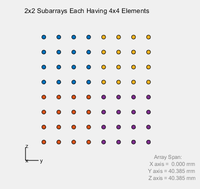
The four elements in one row of a tile cover 3 spacings. One more spacing reaches the first element of the next tile. So 'GridSpacing',4.0*lambda/2 is the value where the tiles join into one continuous grid. The listing below builds that case and draws it with viewArray().

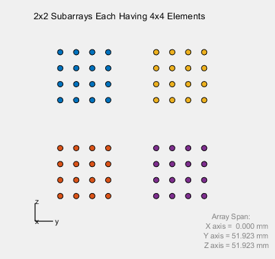
The three plots below show the layout for three grid spacings. The four colours mark the four subarrays. The Array Span note in the lower right gives the size of the whole array along each axis.

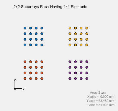
• 4.0*lambda/2 gives one continuous 8 x 8 grid : at 26 GHz, lambda is about 11.54 mm. The span is 4 x 5.77 mm plus 3 x 5.77 mm, which is 40.385 mm. This matches the Y axis and Z axis values in the plot.
• 6.0*lambda/2 opens a gap between the tiles : the centres move 34.6 mm apart, and the span grows to 51.923 mm on both axes.
• A vector sets the two spacings separately : 'GridSpacing',[6.0*lambda/2,8.0*lambda/2] gives the row spacing first and the column spacing second. So the span along z stays at 51.923 mm, and the span along y grows to 63.462 mm.
• The X axis span is 0 : all elements lie in the yz plane, so the array is flat, as the URA is.

What pattern does the replicated array give ?

A replicated array with touching tiles has the same element positions as one big URA. So its pattern should be the pattern of an 8 x 8 URA, and that is a good check before trying anything else. The listing below plots it in 3D with 'Type','powerdB'.

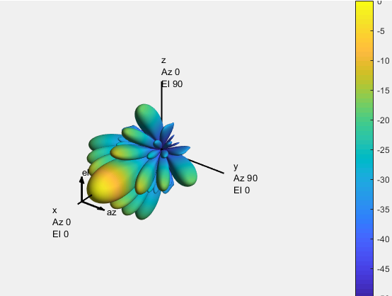
The pattern below uses 'GridSpacing',4.0*lambda/2. The main beam points along x, which is broadside, and the sidelobes form a cross along the y and z axes.

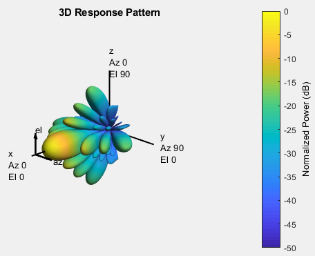
• The pattern matches the 8 x 8 URA : compare it with the 8 x 8 powerdB plot on the URA page. The tiles touch, so the element grid is the same and the pattern is the same.
• The first sidelobe is about -12.8 dB : for 8 elements at lambda/2, the first sidelobe of the array factor is at -12.8 dB. It sits about 21 deg off broadside in each principal plane.
• A gap between tiles creates grating lobes : the page shows only the layout for the wider spacings, but the effect can be computed. With 'GridSpacing',6.0*lambda/2, the subarray centres are 3 lambda apart. In each principal plane, the strongest sidelobe then rises to about -5.9 dB at 16.5 deg. With 8.0*lambda/2, it rises to about -3.4 dB at 13.3 deg.

How is a replicated subarray steered ?

Steering a tiled array needs two phase settings, and it helps to separate them. Each subarray has its own phase shifters, which point the subarray pattern. The array level weights then set the phase between the subarray centres. The beam forms where both point the same way.

The listing below does both. 'SubarraySteering','Phase' tells Matlab that each subarray has phase shifters tuned at 'PhaseShifterFrequency'. 'SteerAngle',steer_ang in pattern() points those phase shifters. The phased.SteeringVector object computes wts_array, one weight per subarray, and 'Weights',wts_array applies it. The steer_ang vector is given as [azimuth; elevation] in degrees.

The first plot below shows the unsteered beam from a different camera angle. The command view(90+37.5,30) moves the camera 37.5 deg from the broadside axis toward the y axis, and 30 deg up. From there, the cross of sidelobes is easier to see.

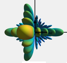
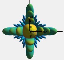
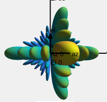
The next two tables steer in azimuth, with elevation fixed at 0. The command view(90,0) puts the camera on the x axis, so you look straight into the broadside direction. In these plots, the beam moves left for -15 deg and right for +15, 30 and 60 deg.

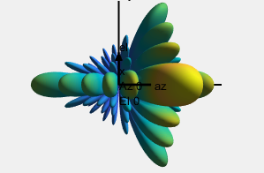
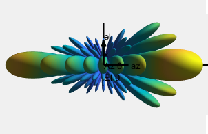
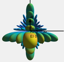
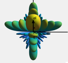
The last two tables steer in elevation, with azimuth fixed at 0. The beam moves down for -15 deg and up for +15, 30, 45 and 60 deg. The sidelobe cross turns with it.

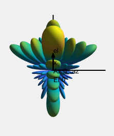
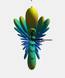
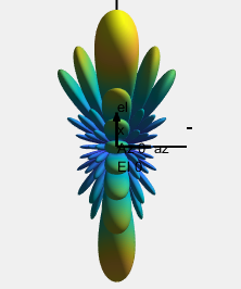
• Both levels must point the same way : if only the subarray centres were steered to 30 deg, the beam would stay at broadside. With touching tiles, sin 30 deg = 0.5 falls exactly on a null of the 4 element subarray pattern. So the array puts no energy there. With 'SubarraySteering','Phase' and 'SteerAngle', the subarray pattern moves too.
• The beam widens as it moves off broadside : for 8 elements at lambda/2, the computed half power beamwidth is 12.8 deg at broadside. It grows to 14.8 deg at 30 deg and 28.8 deg at 60 deg.
• A large lobe appears at the far side at 60 deg : the lobe at the left edge of the 60 deg azimuth plot is the array factor near -90 deg. Its computed level is about -4.5 dB below the peak, as the URA page shows for elevation steering.
• The phase shifters are exact at one frequency only : 'PhaseShifterFrequency',fc sets the frequency where the subarray phase equals the needed delay. Away from fc, the subarray beam points slightly off the array beam.

Disclaimer ! :

This page is only to show you the overall logics and visualization for various Phase Array Antenna System. I haven't investigated much about verifying about the accuracy.

If you think the code is not so efficient, it is 100% my fault. I haven't made any effort for effiecient code. I just tried to create code as simple as possible for the readers. As you know, easy-to-read code is not always efficient for a specific chipset.

If you find any mistake in terms of accuracy, it is also very highly likely be my fault. Not the problem of Matlab tool box itself.

Any comment and corrections if you find any mistake will be welcome and appreciated.