Matlab Toolbox - Antenna
ULA is the Object that is for design and simulating the set of antenna placed along a line. This is the type of array antenna that are used for MIMO (e.g, LTE MIMO).
Every script on this page uses the same setup. The carrier is 26 GHz, the elements are isotropic, and they sit half a wavelength apart along the y axis. Only the element count and the steering angle change from one run to the next, so the plots can be compared directly. I'll start with the numbers behind one beam and then sweep the angle in 2D. After that, we'll look at the full 3D pattern with and without steering.
- Basic Numerical Test
- Plotting Radiation Pattern in 2D
- Plotting Radiation Pattern in 3D
- Steering ULA Pattern in 3D
- Steering ULA Pattern in 2D
Basic Numerical Test
Before any pattern is plotted, let's check what the ULA object and its steering vector actually hold. ULA_Basic_01.m builds a four element array at 26 GHz and prints every intermediate result. The five runs below change only the two red lines, txang and txbeam_ang, so you can compare the printed values directly.
|
ULA_Basic_01.m |
|
c = 3e8; % propagation speed fc = 26e9; % carrier frequency lambda = c/fc; % wavelength
txarray = phased.ULA('NumElements',4,'ElementSpacing',lambda/2) txmipos = getElementPosition(txarray)/lambda
txarraystv = phased.SteeringVector('SensorArray',txarray,'PropagationSpeed',c)
txang = [0 ; 0]; wt = txarraystv(fc,txang)'
txbeam_ang = 0; txsv = steervec(txmipos,txbeam_ang)
txbeam = wt * txsv |
|
txang = [0 ; 0]; txbeam_ang = 0 |
|
txarray =
phased.ULA with properties:
Element: [1×1 phased.IsotropicAntennaElement] NumElements: 4 ElementSpacing: 0.0058 ArrayAxis: 'y' Taper: 1
txmipos =
0 0 0 0 -0.7500 -0.2500 0.2500 0.7500 0 0 0 0
txarraystv =
phased.SteeringVector with properties:
SensorArray: [1×1 phased.ULA] PropagationSpeed: 300000000 IncludeElementResponse: false NumPhaseShifterBits: 0
wt =
1 1 1 1
txsv =
1 1 1 1
txbeam =
4 |
|
txang = [0 ; 0]; txbeam_ang = -10 |
|
txarray =
phased.ULA with properties:
Element: [1×1 phased.IsotropicAntennaElement] NumElements: 4 ElementSpacing: 0.0058 ArrayAxis: 'y' Taper: 1
txmipos =
0 0 0 0 -0.7500 -0.2500 0.2500 0.7500 0 0 0 0
txarraystv =
phased.SteeringVector with properties:
SensorArray: [1×1 phased.ULA] PropagationSpeed: 300000000 IncludeElementResponse: false NumPhaseShifterBits: 0
wt =
1 1 1 1
txsv =
0.6835 + 0.7300i 0.9630 + 0.2694i 0.9630 - 0.2694i 0.6835 - 0.7300i
txbeam =
3.2930 |
|
txang = [0 ; 0]; txbeam_ang = 10 |
|
txarray =
phased.ULA with properties:
Element: [1×1 phased.IsotropicAntennaElement] NumElements: 4 ElementSpacing: 0.0058 ArrayAxis: 'y' Taper: 1
txmipos =
0 0 0 0 -0.7500 -0.2500 0.2500 0.7500 0 0 0 0
txarraystv =
phased.SteeringVector with properties:
SensorArray: [1×1 phased.ULA] PropagationSpeed: 300000000 IncludeElementResponse: false NumPhaseShifterBits: 0
wt =
1 1 1 1
txsv =
0.6835 - 0.7300i 0.9630 - 0.2694i 0.9630 + 0.2694i 0.6835 + 0.7300i
txbeam =
3.2930 |
|
txang = [-10 ; 0]; txbeam_ang = 0 |
|
txarray =
phased.ULA with properties:
Element: [1×1 phased.IsotropicAntennaElement] NumElements: 4 ElementSpacing: 0.0058 ArrayAxis: 'y' Taper: 1
txmipos =
0 0 0 0 -0.7500 -0.2500 0.2500 0.7500 0 0 0 0
txarraystv =
phased.SteeringVector with properties:
SensorArray: [1×1 phased.ULA] PropagationSpeed: 300000000 IncludeElementResponse: false NumPhaseShifterBits: 0
wt =
0.6835 - 0.7300i 0.9630 - 0.2694i 0.9630 + 0.2694i 0.6835 + 0.7300i
txsv =
1 1 1 1
txbeam =
3.2930 |
|
txang = [10 ; 0]; txbeam_ang = 0 |
|
txarray =
phased.ULA with properties:
Element: [1×1 phased.IsotropicAntennaElement] NumElements: 4 ElementSpacing: 0.0058 ArrayAxis: 'y' Taper: 1
txmipos =
0 0 0 0 -0.7500 -0.2500 0.2500 0.7500 0 0 0 0
txarraystv =
phased.SteeringVector with properties:
SensorArray: [1×1 phased.ULA] PropagationSpeed: 300000000 IncludeElementResponse: false NumPhaseShifterBits: 0
wt =
0.6835 + 0.7300i 0.9630 + 0.2694i 0.9630 - 0.2694i 0.6835 - 0.7300i
txsv =
1 1 1 1
txbeam =
3.2930 |
Let's read the first output block from the top. The carrier is 26 GHz, so lambda = c/fc is 11.54 mm and the spacing lambda/2 is 5.77 mm. The object prints this in metres and rounds it to ElementSpacing: 0.0058. The txmipos array holds the same positions divided by lambda, so its middle row reads -0.75, -0.25, 0.25 and 0.75. The first and third rows are zero because the object reports ArrayAxis: 'y'. In other words, the four elements sit on the y axis, half a wavelength apart and centred on the origin.
Figure 1 draws that geometry in the xy plane. A plane wave from azimuth θ reaches neighbouring elements with a path difference of d sinθ. With d = λ/2, that path difference becomes a phase step of π sinθ between neighbours. The azimuth is measured from the x axis, so θ = 0 is broadside.
Figure 1. The ULA built by ULA_Basic_01.m, drawn in the xy plane. Broadside is the x axis, and the phase step between neighbouring elements grows with sinθ, not with θ itself.
- The labels on the left are the txmipos values, so each element position p is in wavelengths.
- The bracket marks the spacing d, which the object prints as ElementSpacing: 0.0058 in metres.
- The red arrow is the direction being tested, txbeam_ang in ULA_Basic_01.m, or the steering direction when it stands for txang.
Next, look at how the beam value is formed. The call steervec(txmipos,txbeam_ang) returns one entry per element, ej2πpnsinθ, where pn is the position in wavelengths. The line wt = txarraystv(fc,txang)' takes the steering vector for txang and applies the apostrophe, which in MATLAB is the conjugate transpose. So txbeam = wt * txsv is an inner product. It measures how well the direction the weights point at matches the direction being tested.
The printed values follow directly. With txang and txbeam_ang both at 0, every term is 1 and txbeam prints 4, the element count. With the two angles 10 degrees apart, the terms no longer line up and txbeam prints 3.2930. That is 0.823 of the peak, or about -1.7 dB in power. The result is real rather than complex because the array is centred on the origin. The phases of each symmetric pair of elements cancel.
Now compare the last four runs. In the second and third runs, wt stays at 1 1 1 1 and txsv carries the phase. In the last two runs the roles swap, so txsv is all ones and wt carries the phase. The magnitude is 3.2930 in all four cases. The reason is that only the difference sinθ - sinθ0 enters the sum, where θ0 is the steering angle. You can also see that the -10 and +10 vectors are complex conjugates of each other, because sin(-θ) = -sinθ.
txbeam peaks at N, not at 1 : four unit weights add coherently to 4. The plotting script in the next section divides by the maximum, so its curves peak at 1.Broadside needs no phase shift : with txang = [0 ; 0], wt is 1 1 1 1. A beam at 0 degrees uses equal weights with no phase.Only the difference in sinθ matters : moving the weights or moving the test angle by the same amount gives the same 3.2930.Two units are in play : ElementSpacing is in metres, while txmipos is in wavelengths. The steervec function expects wavelengths, which is why the script divides by lambda.
Plotting Radiation Pattern in 2D
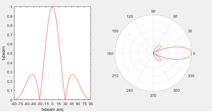
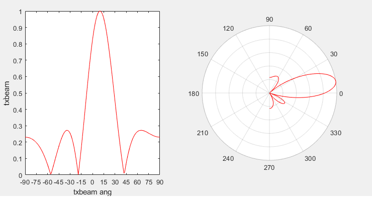
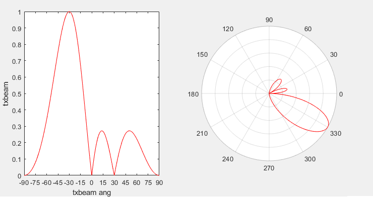
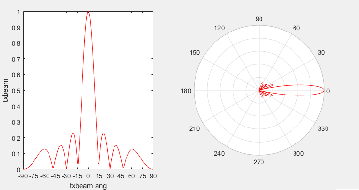
Now let's turn that single number into a curve. ULA_Basic_02.m repeats the same inner product for every txbeam_ang from -90 to 90 degrees and normalises the peak to 1. It draws the result twice, as a Cartesian amplitude plot on the left and a polar plot on the right. Keep in mind that the sweep covers only the front half plane, so the polar plot stays empty behind the array.
|
ULA_Basic_02.m |
|
c = 3e8; % propagation speed fc = 26e9; % carrier frequency lambda = c/fc; % wavelength NoOfTxAntenna = 4
txarray = phased.ULA('NumElements',NoOfTxAntenna,'ElementSpacing',lambda/2); txmipos = getElementPosition(txarray)/lambda;
txarraystv = phased.SteeringVector('SensorArray',txarray,'PropagationSpeed',c);
txang = [0 ; 0]; wt = txarraystv(fc,txang)';
txbeam_ang = -90:90; txbeam_ang_rad = (pi*txbeam_ang)/180; txbeam = abs(wt*steervec(txmipos,txbeam_ang)); txbeam = txbeam/max(txbeam); [txbeampos_x,txbeampos_y] = pol2cart(deg2rad(txbeam_ang),txbeam);
hFig = figure(1); set(hFig, 'Position', [0 0 800 400]); subplot(1,2,1); plot(txbeam_ang,txbeam,'r-'); xlabel('txbeam ang');ylabel('txbeam'); set(gca,'xtick',-90:15:90) xlim([txbeam_ang(1) txbeam_ang(end)]); ylim([0 1.0]); subplot(1,2,2); polarplot(txbeam_ang_rad,txbeam,'r'); set(gca,'RTickLabels',[]); |
Following examples shows the pattern of an array antenna with different steering angles.
|
NoOfTxAntenna = 4 txang = [0 ; 0]; |
|
|
|
NoOfTxAntenna = 4 txang = [10 ; 0]; |
|
|
|
NoOfTxAntenna = 4 txang = [-30 ; 0]; |
|
|
|
NoOfTxAntenna = 8 txang = [0 ; 0]; |
|
|
|
NoOfTxAntenna = 8 txang = [-30 ; 0]; |
|
|
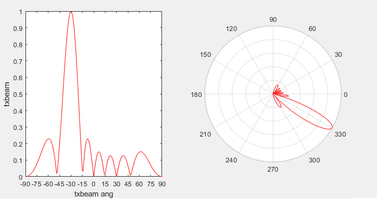
The steered runs above show where the nulls go. For four elements the nulls sit where sinθ - sinθ0 is a multiple of 1/2, and in general a multiple of 2/N. For txang = [10 ; 0] that puts them at -55.7, -19.1 and 42.3 degrees, which is where the curve touches zero. For txang = [-30 ; 0] the nulls land at -90, 0 and 30 degrees. The eight element run at -30 degrees follows the same rule with a step of 1/4 in sinθ. Its nulls fall at both ends of the sweep and at -48.6, -14.5, 0, 14.5, 30 and 48.6 degrees.
Steering also widens the beam. At broadside the four element half power beamwidth is 26.3 degrees, and at -30 degrees it grows to 30.9 degrees. The beam has a fixed width in sinθ, and the same width in sinθ covers more degrees away from broadside. You can also check the two ends of each curve. With half wavelength spacing the pattern repeats every 2 in sinθ - sinθ0. The two ends of the sweep are exactly 2 apart in sinθ. So each curve ends at the same height on both sides, for example 0.23 in the txang = [10 ; 0] run.
Following examples shows how the shape of an array antenna changes as the number of elements increases.
|
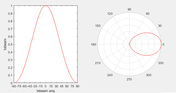
NoOfTxAntenna = 2 txang = [0 ; 0]; |
|
|
|
NoOfTxAntenna = 4 txang = [0 ; 0]; |
|
|
|
NoOfTxAntenna = 8 txang = [0 ; 0]; |
|
|
|
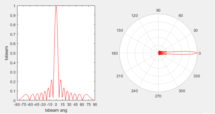
NoOfTxAntenna = 16 txang = [0 ; 0]; |
|
|
Now set the four element counts side by side. The table below is computed for the same half wavelength ULA with uniform weights at broadside, and its values agree with the plots above.
NoOfTxAntenna |
half power beamwidth |
first null |
first sidelobe, amplitude |
first sidelobe, power |
2 |
60.0 deg |
90 deg, endfire |
none |
none |
4 |
26.3 deg |
30.0 deg |
0.27 |
-11.3 dB |
8 |
12.8 deg |
14.5 deg |
0.23 |
-12.8 dB |
16 |
6.4 deg |
7.2 deg |
0.22 |
-13.2 dB |
Three things follow from the table. First, doubling the element count halves the beamwidth. The usual approximation 0.886 λ/(N d) radians is within a degree from four elements upward. At two elements it misses by about 9 degrees. Second, the first null sits at sinθ = 2/N, which is 30 degrees for four elements and 7.2 degrees for sixteen. Third, the first sidelobe barely changes. It moves from -11.3 dB at four elements toward about -13 dB, however many elements are added. Only a non-uniform amplitude taper lowers it, and every array here prints Taper: 1.
Element count sets resolution : each doubling of N halves the beamwidth and halves the sine of the first null angle.Element count does not set the sidelobe level : with uniform weights the first sidelobe stays near -13 dB.Steering costs beamwidth : the same four elements give 26.3 degrees at broadside and 30.9 degrees at 30 degrees off broadside.The polar plot shows only the front half : the sweep stops at plus and minus 90 degrees. The back half appears only in the pattern plots further down.One line in ULA_Basic_02.m is unused : pol2cart computes txbeampos_x and txbeampos_y, but polarplot works from the angle and the magnitude directly.
Plotting Radiation Pattern in 3D
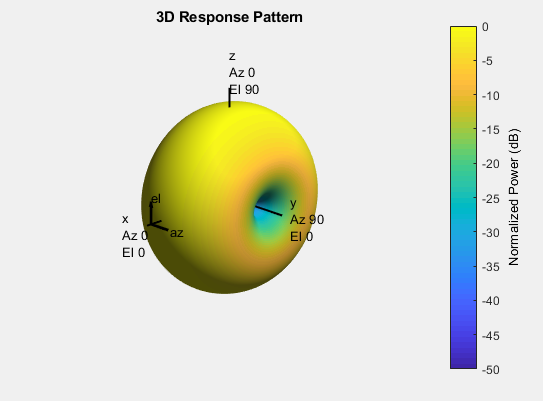
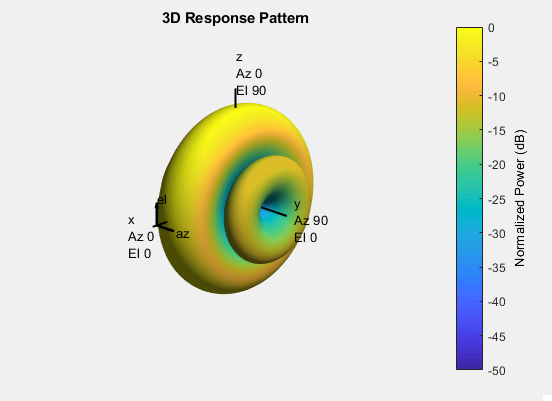
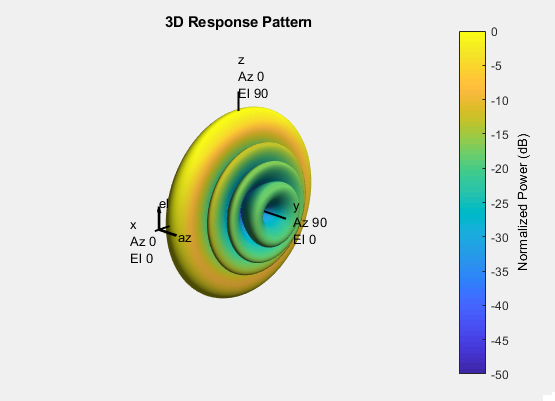
The 2D sweep cuts the pattern along one line. ULA_Basic_03.m asks the toolbox pattern function for every azimuth from -180 to 180 degrees and every elevation from -90 to 90 degrees. So the whole surface appears at once. The surfaces below show normalised power in dB for 2, 4, 8 and 16 elements with no steering.
|
ULA_Basic_03.m |
|
c = 3e8; % propagation speed fc = 26e9; % carrier frequency lambda = c/fc; % wavelength NoOfTxAntenna = 8
txarray = phased.ULA('NumElements',NoOfTxAntenna,'ElementSpacing',lambda/2);
pattern(txarray,fc,[-180:180],[-90:90],... 'PropagationSpeed',c,... 'CoordinateSystem','polar',... 'Type','powerdb') |
|
NoOfTxAntenna = 2 |
|
|
|
NoOfTxAntenna = 4 |
|
|
|
NoOfTxAntenna = 8 |
|
|
|
NoOfTxAntenna = 16 |
|
|
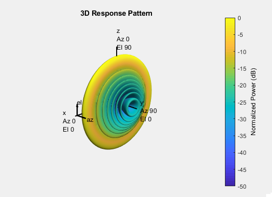
All four surfaces share one property. They are rotationally symmetric about the y axis, which is the array axis printed in the first output. The elements lie on a line, so the array can only tell directions apart by their angle from that line. Every direction at the same angle from y gets the same response.
Now follow the surfaces in order of element count. At two elements the pattern is nearly a sphere with a dimple along y. At four elements one sidelobe ring appears, and at eight and sixteen elements there are three and seven rings. In general a uniform half wavelength array has N/2 - 1 sidelobes between broadside and each end of the axis. The dark spot along y is a true null. For any even N with this spacing, the response in the endfire direction is exactly zero.
Note what does not happen. The main lobe becomes a thinner disc, but it never closes into a spot. A ULA narrows its beam in the plane that contains the array axis and leaves it uniform around that axis. A beam that is narrow in two planes needs elements in two dimensions, as in the URA.
A ULA resolves one angle only : the pattern is a surface of revolution about the y axis.More elements give a thinner disc : the beam narrows toward the xz plane, but it does not become a pencil beam.The colour scale is normalised power in dB : it runs from 0 at the peak to -50. The rings are sidelobes, and the dark spot on the y axis is the endfire null.
Steering ULA Pattern in 3D
Now let's steer the 3D pattern. ULA_Basic_04.m builds weights for steer_ang with phased.SteeringVector and hands them to pattern through the 'Weights' option. The call view(90,0) puts the camera on the +x axis, which is broadside. So the y axis runs from left to right across each picture. Each image table states in its header row whether it plots 'powerdb' or linear 'power'.
|
ULA_Basic_04.m |
|
c = 3e8; fc = 26e9; lambda = c/fc;
NoOfTxAntenna = 4;
txarray = phased.ULA('NumElements',NoOfTxAntenna,'ElementSpacing',lambda/2); steer_ang = [15;0]; stv = phased.SteeringVector('SensorArray',txarray); w = stv(fc,steer_ang);
pattern(txarray,fc,[-180:180],[-90:90],... 'PropagationSpeed',c,... 'CoordinateSystem','polar',... 'Type','powerdb',... 'Weights',w)
view(90,0); |
|
steer_ang = [-15;0]; 'Type','powerdb' view(90,0); |
steer_ang = [0;0]; 'Type','powerdb' view(90,0); |
steer_ang = [15;0]; 'Type','powerdb' view(90,0); |
|
|
|
|


|
steer_ang = [30;0]; 'Type','powerdb' view(90,0); |
steer_ang = [45;0]; 'Type','powerdb' view(90,0); |
steer_ang = [60;0]; 'Type','powerdb' view(90,0); |
|
|
|
|


|
steer_ang = [-15;0]; 'Type','power' view(90,0); |
steer_ang = [0;0]; 'Type','power' view(90,0); |
steer_ang = [15;0]; 'Type','power' view(90,0); |
|
|
|
|


|
steer_ang = [30;0]; 'Type','power' view(90,0); |
steer_ang = [45;0]; 'Type','power' view(90,0); |
steer_ang = [60;0]; 'Type','power' view(90,0); |
|
|
|
|


|
steer_ang = [30;0]; 'Type','power' view(90,0); |
steer_ang = [30;0]; 'Type','power' view(120,0); |
steer_ang = [30;0]; 'Type','power' view(90,0); |
|
|
|
|


Start with the 'powerdb' pictures. At steer_ang = [0;0] the main lobe is the tall body in the middle. The two smaller bodies on either side are the sidelobe ring seen edge on. As steer_ang grows, the main lobe moves to the right, toward +y. At -15 degrees it moves to the left instead. The dB scale makes the sidelobes look almost as large as the main lobe, although they are 11.3 dB down.
The linear 'power' pictures look different. In linear power the sidelobes are 0.074 of the peak, so they almost disappear. At broadside the main lobe is a thin disc seen edge on. When the beam is steered, the disc bends into a cone that opens toward +y. The half angle of that cone, measured from the y axis, is 90 degrees minus the steering angle. For steer_ang of 15, 30, 45 and 60 degrees it is 75, 60, 45 and 30 degrees.
The -y side needs attention at large angles. At 45 degrees a small lobe appears on the left, along -y. At 60 degrees that lobe reaches -1 dB, which is 0.80 of the peak power. This is the grating lobe of the half wavelength array starting to enter visible space. The pattern repeats every 2 in sinθ, so a beam at sinθ0 = 0.87 has a copy at -1.13, just outside the visible range. The skirt of that copy lifts the response at -90 degrees. So a four element half wavelength ULA steered to 60 degrees radiates almost as strongly along -y as in the intended direction.
The image table whose middle header reads view(120,0) shows one pattern from three cameras. All three file names say Steering_30, and the shapes match the 30 degree cone. The middle picture follows view(120,0), so the cone is seen partly from its open end. The right picture looks straight down the +y axis, and its dark centre is the null that a 30 degree beam puts along y. The header cells of the middle and right pictures first read steer_ang = [45;0] and [60;0], copied from the table above, and now read [30;0] to match the pictures. The right cell still reads view(90,0), although its picture looks along the y axis, so that camera setting is probably a leftover as well.
One small detail in ULA_Basic_04.m is the propagation speed. The phased.SteeringVector object is created without 'PropagationSpeed', so it uses the default speed of light, 299792458 m/s, while pattern uses c = 3e8. The weights therefore point about 0.07 degrees away from steer_ang at 60 degrees, which is far below what the plots can show.
Steering bends the disc into a cone : off broadside, a ULA radiates on a cone around the y axis. It does not radiate in a single direction.Linear power hides the sidelobes : at -11.3 dB they are 0.074 of the peak. Compare 'power' and 'powerdb' before judging a pattern by its shape.Large steering angles raise the response along -y : at 60 degrees that response is only 1 dB below the peak.
Steering ULA Pattern in 2D
The 3D surfaces are hard to read numerically, so ULA_Basic_05.m takes one slice of them. It plots the azimuth cut at elevation 0 in polar and rectangular form, both in dB, for steering angles from -5 to 60 degrees. The rectangular plot on the right is the easier one to read values from.
|
ULA_Basic_05.m |
|
c = 3e8; fc = 26e9; lambda = c/fc;
NoOfTxAntenna = 4;
txarray = phased.ULA('NumElements',NoOfTxAntenna,'ElementSpacing',lambda/2); steer_ang = [-5;0]; stv = phased.SteeringVector('SensorArray',txarray); w = stv(fc,steer_ang);
subplot(1,2,1); pattern(txarray,fc,[-180:180],0,... 'PropagationSpeed',c,... 'CoordinateSystem','polar',... 'Type','powerdb',... 'Weights',w)
subplot(1,2,2); pattern(txarray,fc,[-180:180],0,... 'PropagationSpeed',c,... 'CoordinateSystem','rectangular',... 'Type','powerdb', ... 'Weights',w)
set(gcf, 'Position', [200, 200, 740, 350]) |
|
NoOfTxAntenna = 4; steer_ang = [-5;0]; 'Type','powerdB' |
|
|

|
NoOfTxAntenna = 4; steer_ang = [0;0]; 'Type','powerdB' |
|
|

|
NoOfTxAntenna = 4; steer_ang = [5;0]; 'Type','powerdB' |
|
|

|
NoOfTxAntenna = 4; steer_ang = [10;0]; 'Type','powerdB' |
|
|

|
NoOfTxAntenna = 4; steer_ang = [15;0]; 'Type','powerdB' |
|
|

|
NoOfTxAntenna = 4; steer_ang = [30;0]; 'Type','powerdB' |
|
|

|
NoOfTxAntenna = 4; steer_ang = [45;0]; 'Type','powerdB' |
|
|

|
NoOfTxAntenna = 4; steer_ang = [60;0]; 'Type','powerdB' |
|
|

Unlike the sweep in ULA_Basic_02.m, this cut covers the full circle from -180 to 180 degrees, so the back half of the pattern appears. Azimuths θ and 180 - θ have the same sinθ, and a line of isotropic elements cannot tell them apart. Every lobe therefore appears twice, once in front of the array and once mirrored behind it. At steer_ang = [0;0] the peaks sit at 0 and 180 degrees, and the sidelobes are near -11 dB. The nulls sit at plus or minus 30, 90 and 150 degrees.
Small steering angles move the front lobe and its mirror in opposite directions. At 5 degrees the main lobe sits at 5 degrees and its mirror at 175 degrees. The nulls move too, to -155.6, -114.1, -65.9, -24.4, 36.0 and 144.0 degrees, and the rectangular plot shows them there. At -5 degrees the same nulls appear with the sign reversed.
At larger angles the two lobes meet at 90 degrees. At 30 degrees they are still separate, with peaks at 30 and 150 degrees and a deep null at 90 degrees between them. At 45 degrees they merge into one broad hump with only a -5.3 dB dip at 90 degrees. At 60 degrees the dip is about -1 dB. At the same time the lobe around -90 degrees rises, to -5.3 dB at 45 degrees and -1 dB at 60 degrees. This is the same lobe that the linear power plots in the previous section show along -y.
A ULA has a front and back ambiguity : with isotropic elements, every lobe at θ has a twin at 180 - θ.Nulls follow sinθ, not θ : for four elements they sit where sinθ - sinθ0 is a multiple of 1/2.Past about 45 degrees the front lobe is no longer a separate beam : it merges with its mirror at 90 degrees. The lobe at -90 degrees also rises to within a few dB of the peak.