Matlab Toolbox - Antenna
A uniform rectangular array, URA, places identical antenna elements on a regular grid. A linear array can steer its beam in one plane only. A grid has elements along two axes, so it can form a narrow beam and steer it in both azimuth and elevation. This page builds URAs of several sizes in Matlab, plots their patterns, and then steers the beam with a steering vector. The carrier is 26 GHz and the element spacing is half a wavelength in every example.
It is required to have Matlab Phased Array System Toolbox to run the examples shown here.
All the sample plots shown here are based on the code URA_Basic_01.m which use Isotropic Antenna as elements of the antenna array. If you want to use different type of antenna element (e.g, CrossedDipole), you may specify the Antenna Element as shown in URA_Basic_02.m.
- How is a URA defined in Matlab ?
- What does each pattern Type show ?
- How does the array size change the beam ?
- Steering of URA in 3D Pattern
- Steering of URA in 2D Pattern
How is a URA defined in Matlab ?
Before reading the plots, you need to know how Matlab places the elements. The phased.URA object takes 'Size' as [rows columns]. The rows run along the z axis, and the columns run along the y axis. So the array lies in the yz plane. Its broadside direction is the x axis, which is azimuth 0 deg and elevation 0 deg in every plot below.
'ElementSpacing' is also given as [row spacing, column spacing]. At fc = 26 GHz, lambda is about 11.5 mm, so lambda/2 is about 5.8 mm. An 8 x 8 array is therefore only about 46 mm on each side. The default element is an isotropic antenna. BackBaffled = true removes its radiation toward the back, at azimuth beyond +/-90 deg. A panel with a ground plane does the same.
|
URA_Basic_01.m |
|
c = 3e8; % propagation speed fc = 26e9; % carrier frequency lambda = c/fc; % wavelength
txarray = phased.URA('Size',[8 8],'ElementSpacing',[lambda/2 lambda/2]); txarray.Element.BackBaffled = true;
pattern(txarray,fc,[-180:180],[-90:90],... 'PropagationSpeed',c,... 'CoordinateSystem','polar',... 'Type','powerdB') |
The listing below is the same array with a crossed dipole as the element. A crossed dipole combines two orthogonal dipoles, so it can radiate circular polarization. Polarization = 'RHCP' selects right hand circular polarization. The plots on the rest of the page all come from the isotropic version above, not from this one.
|
URA_Basic_02.m |
|
c = 3e8; % propagation speed fc = 26e9; % carrier frequency lambda = c/fc; % wavelength
antennaElement = phased.CrossedDipoleAntennaElement; txarray = phased.URA('Size',[8 8],'ElementSpacing',[lambda/2 lambda/2] ... ,'Element',antennaElement); txarray.Element.Polarization = 'RHCP'; txarray.Element.RotationAngle = 0;
pattern(txarray,fc,[-180:180],[-90:90],... 'PropagationSpeed',c,... 'CoordinateSystem','polar',... 'Type','powerdB') |
Size is rows by columns, not x by y : 'Size',[8 2] puts 8 elements along z and 2 along y. The rest of the page depends on this. The long side of the array makes the beam narrow.The element sets the pattern far from broadside : an isotropic element leaves the array factor alone. A crossed dipole multiplies it by its own pattern and adds a polarization.Half wavelength spacing keeps grating lobes away : at lambda/2, no second main lobe appears at broadside. The Steering sections below show how close one comes at 60 deg.
What does each pattern Type show ?
The same 8 x 8 array can be plotted in four ways, and the choice changes what you notice. The 'Type' argument of pattern() selects the quantity. A dB scale shows the sidelobes, while a linear scale shows how much of the energy the main lobe holds.
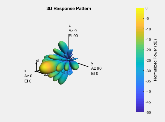
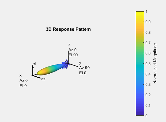
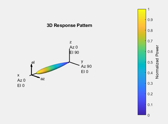
The four plots below show one pattern. In the first, the color bar is normalized power in dB down to -50 dB. In the second and third, it is the normalized magnitude and the normalized power on a linear scale from 0 to 1. The last one is directivity in dBi.
Two numbers link the linear scales and the dB scale. A point at 0.5 on the efield plot sits at 0.25 on the power plot, and at -6 dB on the powerdB plot. The half power edge of the beam sits at 0.707 on the efield scale and 0.5 on the power scale. Both are -3 dB.
|
'Type','powerdB' |
|
|
|
'Type','efield' |
|
|
|
'Type','power' |
|
|
|
'Type','directivity' |
|
|
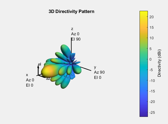
Each Type answers a different question, so the choice depends on the job. Use powerdB to read sidelobe levels and null positions, because only a log scale shows them. Use power or efield to judge the beam shape at a glance, because the sidelobes drop out. Use directivity when the number goes into a link budget, since EIRP is the transmit power plus the directivity in dBi. A simple aperture check confirms the directivity plot. The 8 x 8 array at lambda/2 spacing covers an area of 16 lambda2, and 4π times that area is about 201, or 23.0 dBi. That estimate is close to the 22.8 dBi from the full calculation.
powerdB shows every sidelobe : a -30 dB sidelobe is still a large shape on a 50 dB range. So the whole grid of sidelobes stays visible.efield and power hide the sidelobes : in linear power, a -13 dB sidelobe is only 5 percent of the peak. So the plot looks like one clean beam. The power plot looks narrower than the efield plot, because power is the square of the field magnitude.directivity gives an absolute number : the color bar peaks near 23 dBi. Numerical integration of the array factor gives 22.8 dBi for these back baffled isotropic elements. That matches the plot.
How does the array size change the beam ?
A bigger array gives a narrower beam, but a URA has two sizes, one per axis. Let's change the number of rows and the number of columns separately and see which dimension of the beam each one controls. All plots in this section use powerdB and no steering.
The listing below changes only the 'Size' argument. Its header repeats the name URA_Basic_02.m, which the crossed dipole listing above already uses. The code is the isotropic URA_Basic_01.m with 'Size',[8 2]; the tables that follow change the size in the same place.
|
URA_Basic_02.m |
|
c = 3e8; % propagation speed fc = 26e9; % carrier frequency lambda = c/fc; % wavelength
txarray = phased.URA('Size',[8 2],'ElementSpacing',[lambda/2 lambda/2]); txarray.Element.BackBaffled = true;
pattern(txarray,fc,[-180:180],[-90:90],... 'PropagationSpeed',c,... 'CoordinateSystem','polar',... 'Type','powerdB') |
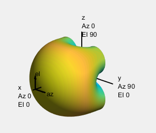
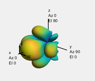
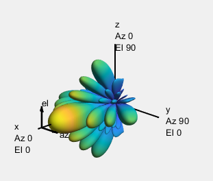
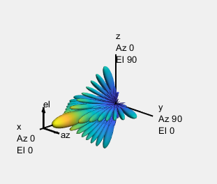
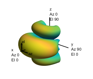
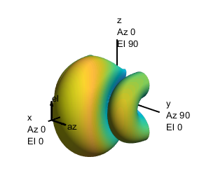
The first table compares square arrays of 2 x 2, 4 x 4, 8 x 8 and 16 x 16. The next two compare rectangular arrays with the row and column counts swapped. They are 4 x 2 against 2 x 4, and 8 x 2 against 2 x 8.
|
'Size',[2 2] |
'Size',[4 4] |
|
|
|
|
'Size',[8 8] |
'Size',[16 16] |
|
|
|
|
'Size',[4 2] |
'Size',[2 4] |
|
|
|
|
'Size',[8 2] |
'Size',[2 8] |
|
|
|
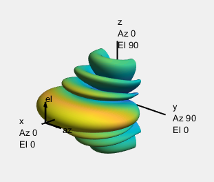
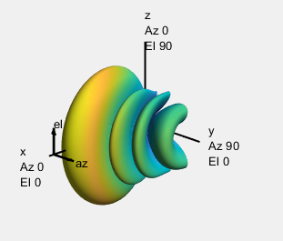
The square arrays narrow the beam in both planes : the 2 x 2 pattern is a broad dome. The 16 x 16 pattern is a thin pencil beam with many small sidelobes. The computed directivity grows from about 10.1 dBi to 16.5, 22.8 and 28.9 dBi. That is 6 dB each time both sides double.The long side narrows the beam in its own plane : 8 x 2 has 8 elements along z. So its beam is narrow in elevation and wide in azimuth. Its sidelobes stack up and down like disks. 2 x 8 is the same pattern turned by 90 deg, narrow in azimuth with sidelobes spread sideways.A fan beam comes from a long, thin array : an array for vertical tilt is tall and narrow. An array for horizontal steering is wide.
To read the beamwidths, it is easier to cut the 3D pattern along one plane. The listing below plots two cuts of a 2 x 8 array. One is an azimuth cut at elevation 0 deg. The other is an elevation cut at azimuth 0 deg.
|
URA_Basic_03.m |
|
c = 3e8; % propagation speed fc = 26e9; % carrier frequency lambda = c/fc; % wavelength
txarray = phased.URA('Size',[2 8],'ElementSpacing',[lambda/2 lambda/2]); txarray.Element.BackBaffled = true;
subplot(1,2,1); pattern(txarray,fc,[-180:180],0,... 'PropagationSpeed',c,... 'CoordinateSystem','polar',... 'Type','powerdB')
subplot(1,2,2); pattern(txarray,fc,0,[-90:90],... 'PropagationSpeed',c,... 'CoordinateSystem','polar',... 'Type','powerdB') |
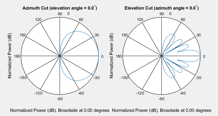
The plots below show both cuts, first for 8 x 2 and then for 2 x 8. In each figure, the left plot is the azimuth cut and the right plot is the elevation cut.
|
'Size',[8 2] |
|
|
|
'Size',[2 8] |
|
|
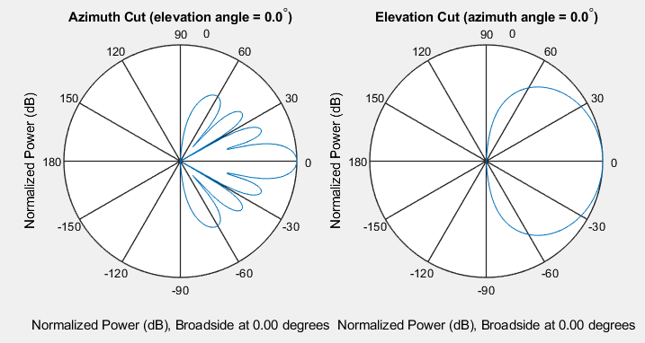
The 8 element cut shows the narrow beam and its sidelobes : the elevation cut of 8 x 2 has a narrow main lobe with three sidelobes on each side. For an 8 element line at lambda/2, the half power beamwidth is 12.8 deg.The 2 element cut is broad : the azimuth cut of 8 x 2 is one wide lobe. The back baffle removes everything behind the array.The two arrays swap their cuts : 2 x 8 shows the same two shapes with azimuth and elevation exchanged.
Steering of URA in 3D Pattern
So far, every beam has pointed at broadside. Let's now point it somewhere else without moving the array. The phased.SteeringVector object computes one complex weight per element for a given direction. Passing those weights to pattern() with 'Weights',w applies the progressive phase shift that steers the beam.
steer_ang is given as [azimuth; elevation] in degrees. The listing keeps azimuth at 0 and changes the elevation. So the 8 x 2 array steers along its 8 element axis, where the beam is narrow.
|
URA_Basic_04.m |
|
c = 3e8; % propagation speed fc = 26e9; % carrier frequency lambda = c/fc; % wavelength
txarray = phased.URA('Size',[8 2],'ElementSpacing',[lambda/2 lambda/2]); txarray.Element.BackBaffled = true;
steer_ang = [0;0]; stv = phased.SteeringVector('SensorArray',txarray); w = stv(fc,steer_ang);
pattern(txarray,fc,[-180:180],[-90:90],... 'PropagationSpeed',c,... 'CoordinateSystem','polar',... 'Type','powerdB', ... 'Weights',w)
view(90,0);,'polar',... 'Type','powerdB') |
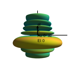
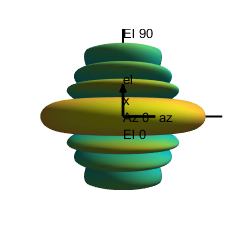
The last two lines of the listing, view(90,0);,'polar',... and 'Type','powerdB'), are left over from an edit. Matlab stops with a parse error on the extra closing parenthesis. Delete both and keep view(90,0);, which turns the camera so the elevation angle runs straight up the picture. The tables below show the pattern for elevation steering from -15 deg to 60 deg in powerdB.
|
BackBaffled = true; steer_ang = [0;-15]; 'Type','powerdB' view(90,0); |
BackBaffled = true; steer_ang = [0;0]; 'Type','powerdB' view(90,0); |
BackBaffled = true; steer_ang = [0;15]; 'Type','powerdB' view(90,0); |
|
|
|
|
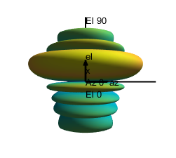
|
BackBaffled = true; steer_ang = [0;30]; 'Type','powerdB' view(90,0); |
BackBaffled = true; steer_ang = [0;45]; 'Type','powerdB' view(90,0); |
BackBaffled = true; steer_ang = [0;60]; 'Type','powerdB' view(90,0); |
|
|
|
|
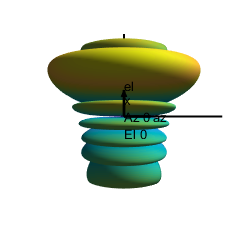
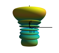
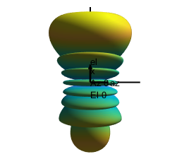
The next two tables repeat the same steering angles with 'Type','power'. A linear scale hides the sidelobes, so the tilt of the main beam is easier to see.
|
BackBaffled = true; steer_ang = [0;-15]; 'Type','power' view(90,0); |
BackBaffled = true; steer_ang = [0;0]; 'Type','power' view(90,0); |
BackBaffled = true; steer_ang = [0;15]; 'Type','power' view(90,0); |
|
|
|
|
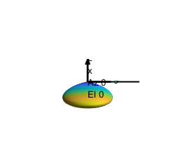
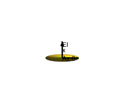
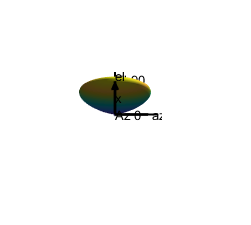
The same beams look different from another camera angle. The table below uses view(-50,-10), which looks at the pattern from the side and slightly below. The beam rises toward the upper right as the elevation grows.
|
BackBaffled = true; steer_ang = [0;30]; 'Type','power' view(90,0); |
BackBaffled = true; steer_ang = [0;45]; 'Type','power' view(90,0); |
BackBaffled = true; steer_ang = [0;60]; 'Type','power' view(90,0); |
|
|
|
|
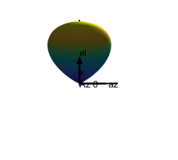
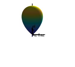
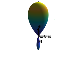
The last 3D table sets BackBaffled to false. The array lies in the yz plane. So it cannot tell a direction in front of the plane from its mirror image behind it. Without the baffle, every beam therefore has a twin pointing toward the back at the same elevation.
|
BackBaffled = true; steer_ang = [0;30]; 'Type','power' view(-50,-10); |
BackBaffled = true; steer_ang = [0;45]; 'Type','power' view(-50,-10); |
BackBaffled = true; steer_ang = [0;60]; 'Type','power' view(-50,-10); |
|
|
|
|


|
BackBaffled = true; steer_ang = [0;30]; 'Type','power' view(-50,-10); |
BackBaffled = true; steer_ang = [0;45]; 'Type','power' view(-50,-10); |
BackBaffled = true; steer_ang = [0;60]; 'Type','power' view(-50,-10); |
|
|
|
|


The beam follows steer_ang : the main lobe rises with the elevation angle in every view.A lobe appears at the bottom at 60 deg : the small lobe below the array in the 60 deg plots is not an error. For this steering angle, the array factor at elevation -90 deg is only 4.5 dB below the peak. The 2D section shows it.Without a back baffle, a planar array radiates a mirrored beam : a real panel uses a ground plane. The ground plane plays the role of BackBaffled = true.
Steering of URA in 2D Pattern
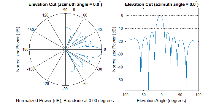
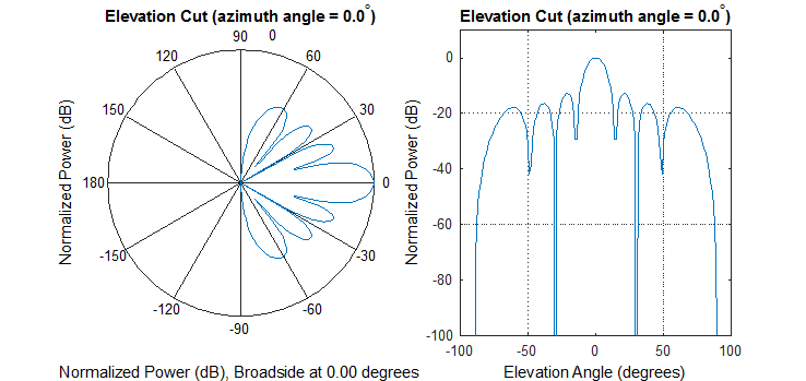
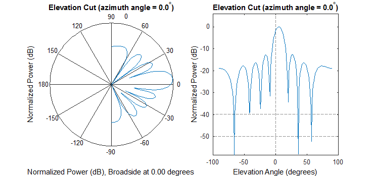
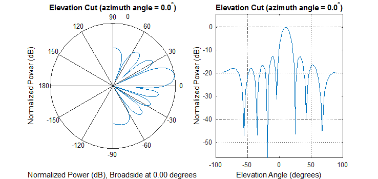
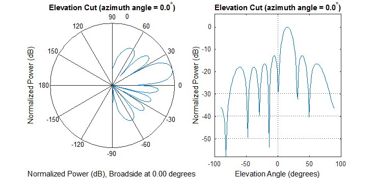
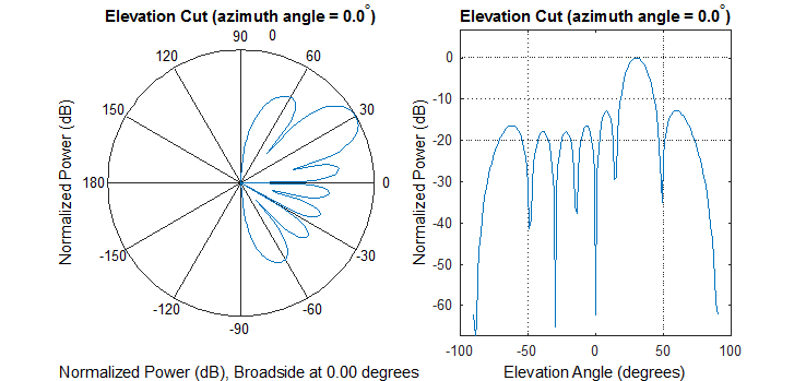
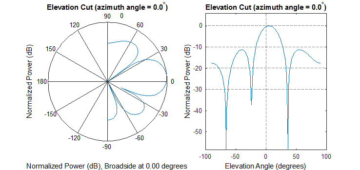
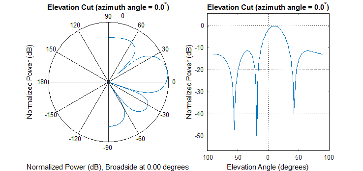
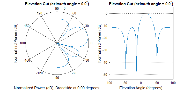
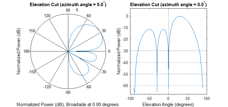
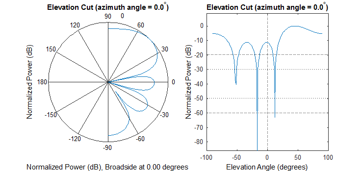
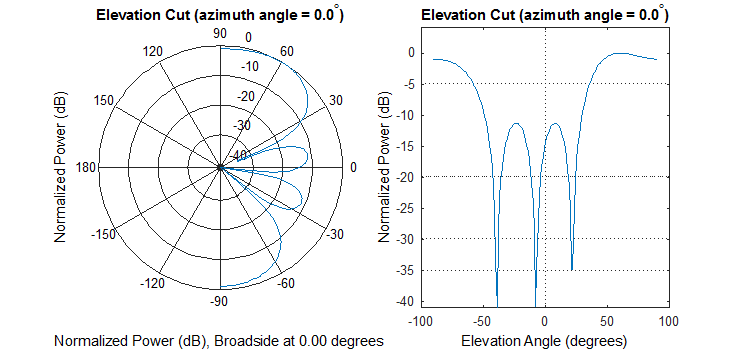
A 3D plot shows where the beam goes, but it is hard to read a level or a beamwidth from it. The elevation cut plots below make both readable. Each figure shows the same cut twice. The left plot is in polar form. The right plot is in rectangular form, with elevation on the horizontal axis.
|
URA_Basic_05.m |
|
c = 3e8; % propagation speed fc = 26e9; % carrier frequency lambda = c/fc; % wavelength
txarray = phased.URA('Size',[8 2],'ElementSpacing',[lambda/2 lambda/2]); txarray.Element.BackBaffled = false;
steer_ang = [0;10]; stv = phased.SteeringVector('SensorArray',txarray); w = stv(fc,steer_ang);
subplot(1,2,1); pattern(txarray,fc,0,[-90:90],... 'PropagationSpeed',c,... 'CoordinateSystem','polar',... 'Type','powerdb', ... 'Weights',w)
subplot(1,2,2); pattern(txarray,fc,0,[-90:90],... 'PropagationSpeed',c,... 'CoordinateSystem','rectangular',... 'Type','powerdb', ... 'Weights',w)
set(gcf, 'Position', [200, 200, 740, 350]) |
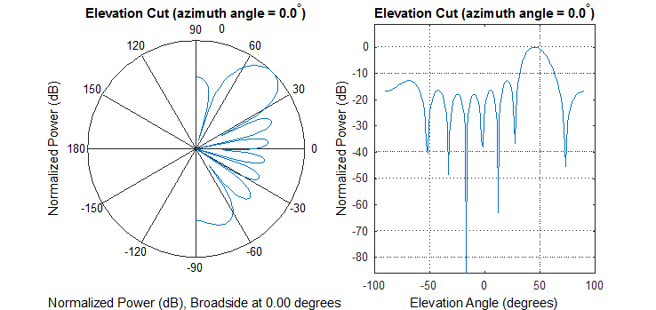
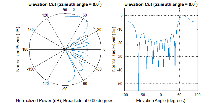
The first eight tables use the 8 x 2 array, steered from -5 deg to 60 deg. The main lobe moves to the steering angle in every plot. It also grows wider as the beam moves away from broadside, because the array looks shorter from that direction.
|
'Size',[8 2] BackBaffled = false; steer_ang = [0;-5]; 'Type','powerdB' |
|
|
|
'Size',[8 2] BackBaffled = false; steer_ang = [0;0]; 'Type','powerdB' |
|
|
|
'Size',[8 2] BackBaffled = false; steer_ang = [0;5]; 'Type','powerdB' |
|
|
|
'Size',[8 2] BackBaffled =false; steer_ang = [0;10]; 'Type','powerdB' |
|
|
|
'Size',[8 2] BackBaffled = false; steer_ang = [0;15]; 'Type','powerdB' |
|
|
|
'Size',[8 2] BackBaffled = false; steer_ang = [0;30]; 'Type','powerdB' |
|
|
|
'Size',[8 2] BackBaffled = false; steer_ang = [0;45]; 'Type','powerdB' |
|
|
|
'Size',[8 2] BackBaffled = false; steer_ang = [0;60]; 'Type','powerdB' |
|
|
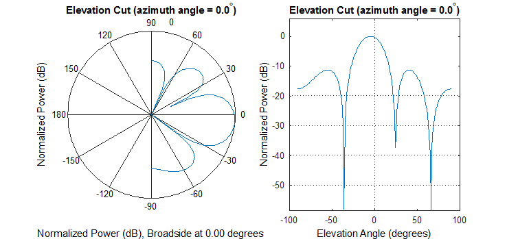
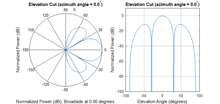
The next eight tables repeat the same angles with the 4 x 2 array. With 4 elements along z, the beam is about twice as wide. Its sidelobes are fewer and higher, and the steering effects show up at smaller angles.
|
'Size',[4 2] BackBaffled = false; steer_ang = [0;-5]; 'Type','powerdB' |
|
|
|
'Size',[4 2] BackBaffled = false; steer_ang = [0;0]; 'Type','powerdB' |
|
|
|
'Size',[4 2] BackBaffled = false; steer_ang = [0;5]; 'Type','powerdB' |
|
|
|
'Size',[4 2] BackBaffled = false; steer_ang = [0;10]; 'Type','powerdB' |
|
|
|
'Size',[4 2] BackBaffled = false; steer_ang = [0;15]; 'Type','powerdB' |
|
|
|
'Size',[4 2] BackBaffled = false; steer_ang = [0;30]; 'Type','powerdB' |
|
|
|
'Size',[4 2] BackBaffled = false; steer_ang = [0;45]; 'Type','powerdB' |
|
|
|
'Size',[4 2] BackBaffled = false; steer_ang = [0;60]; 'Type','powerdB' |
|
|
The table below compares the two arrays with numbers. It is computed from the array factor of the 8 or 4 elements along z, with lambda/2 spacing and uniform weights. The last two columns give the level at elevation -90 deg, below the peak.
Steering angle |
8 x 2 beamwidth |
4 x 2 beamwidth |
8 x 2 level at -90 deg |
4 x 2 level at -90 deg |
0 deg |
12.8 deg |
26.3 deg |
null |
null |
15 deg |
13.3 deg |
27.3 deg |
-36.5 dB |
-11.3 dB |
30 deg |
14.8 deg |
30.9 deg |
null |
null |
45 deg |
18.4 deg |
40.6 deg |
-16.8 dB |
-5.3 dB |
60 deg |
28.8 deg |
50.3 deg |
-4.5 dB |
-1.0 dB |
The beamwidth grows with the steering angle : the 8 x 2 beam goes from 12.8 deg at broadside to 28.8 deg at 60 deg. The 4 x 2 array starts twice as wide and stays about twice as wide.A lobe rises at -90 deg for large steering angles : at 60 deg, the phase step between elements is 0.87 pi. At elevation -90 deg, the total step is 1.87 pi, which is close to a full grating lobe at 2 pi. The 4 x 2 plot shows this lobe at about -1 dB, and the 8 x 2 plot at about -4.5 dB.Keep the steering range inside the sector the array can serve : a wider beam costs gain in the wanted direction. So does a large lobe toward the ground.
Disclaimer !
This page is only to show you the overall logics and visualization for various Phase Array Antenna System. I haven't investigated much about verifying about the accuracy.
If you think the code is not so efficient, it is 100% my fault. I haven't made any effort for effiecient code. I just tried to create code as simple as possible for the readers. As you know, easy-to-read code is not always efficient for a specific chipset.
If you find any mistake in terms of accuracy, it is also very highly likely be my fault. Not the problem of Matlab tool box itself.
Any comment and corrections if you find any mistake will be welcome and appreciated.