Sensitivity is an indicator showing how well a device receive the signal and decode it within a 'satisfactory error rate'. (How low the error rate should be for 'satisfactory error rate' is normally defined by a specification of each application). Sensitivity is represented in a power level (e.g, -100 dBm).

So the interpretation of the sensitivity value goes like this. Let's assume that you (or specification) set BER 1 % to be the level of 'satisfactory error rate'. and assume that the sensitivity of your device is measured to be -100 dBm. This means that the reciever power level down to -100 dBm, BER measured by the device is lower than 1% and if the reciever power gets lower than -100 dBm, the BER gets larger than 1%.

 Here goes another case. Let's assume that you have two device (Device A and B). Device A has the sensitivity of -100 dBm and device B has the sensitivity of -110 dBm. In this case, we can say "Device B has better sensitivity and better reception capability".

Keep the sign in mind when you compare two numbers. Sensitivity is a negative dBm value, so a more negative number is the better one. A 10 dB difference, as between Device A and Device B above, is a factor of 10 in received power. The sections below show how the number is measured, how it can be estimated from NF, bandwidth and SNR, and which conditions LTE uses to make the number comparable between devices.

• How to measure ?
• Estimation of Sensitivity / Factors affecting the Sensitivity
• Conditions for Sensitivity Measurement
• Reference

How to measure ?

Now let's think about how to measure the sensitivity of a device. There are a couple of different ways of measuring the sensitivity, but the most common method is as illustrated below. In both case, we use a specific test equipment which can communicate with the specific DUT with same protocol. For example, if the DUT is a bluetooth device, we use a test equipment which is working in bluetooth protocol (e.g, Anritsu MT8852) and if the DUT is WCDMA device, the test equipment which is supporting WCDMA protocol (e.g, NodeB simulator like Anritsu MT8820 or R&S CMW 500)

There can be two different setups to measure sensitivity using these equipments. In the setup shown on the left, the test equipment transmit the test signal (a known bit sequence) and DUT compares the received bit sequence with the bit sequence generated internally and calculate BER (Bit Error Rate). In the setup shown on the right, the test equipment transmit a bit sequence and UE recieves and retransmit (loopback) the received sequence to the equipment, and the equipment compares the transmitted bit sequence and loopbacked bit sequence and calculate the BER.

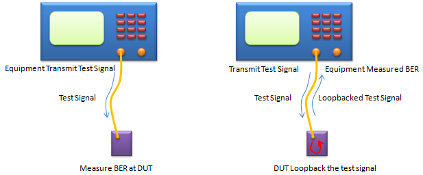
Two ways to count bit errors. The left setup needs a BER counter inside the DUT. The right setup needs only a loopback in the DUT.

• In the left setup, the arrow labelled Test Signal goes one way only, from the equipment to the DUT. The label at the DUT reads Measure BER at DUT.
• In the right setup, the signal goes down as Test Signal and comes back as Loopbacked Test Signal. The label at the equipment reads Equipment Measured BER.
• The loopback setup puts the uplink into the measurement as well. So the uplink must be clean enough to add no errors of its own.

Usually we cannot figure out the sensitivity in a single step and have to repeat the measurement procedure described above multiple steps with different power level. For example, you can measure BER as explained above with power level -40 dBm and measure BER and write down the value. Next, do the same measurement at power level -41 dBm. Repeat this process all to way down to -110 dBm. If you plot the test result, you would see a plot as shown on the right. In this plot, you can find a point (Power level) where BER gets greater than the specified criteria. That power is called 'Sensitivity'.

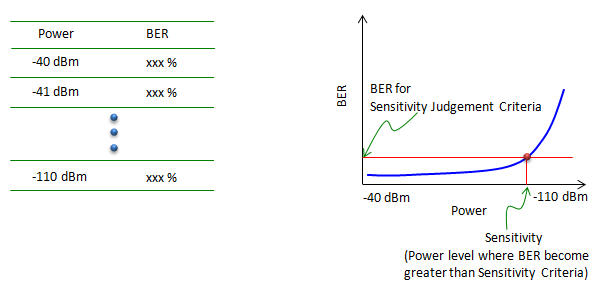
The sensitivity is the power where the BER curve crosses the criteria line. Above that power the BER stays low and almost flat.

• The table on the left lists the power in 1 dB steps, from -40 dBm down to -110 dBm, with the BER measured at each step.
• In the plot, power decreases from -40 dBm at the left to -110 dBm at the right. The BER stays near the floor over most of the range and rises steeply near the low end.
• The horizontal line is labelled BER for Sensitivity Judgement Criteria. The red dot where the curve crosses it is labelled Sensitivity.

The steep part of the curve is the reason a 1 dB step is usually enough. Near the sensitivity point, a few dB of power change moves the BER by a large factor. So a coarse sweep can find the region quickly, and a finer sweep around the crossing can refine the value. Automated test systems often use a search rather than a full sweep for the same reason.

• Sensitivity is a threshold, not a single measurement : it is the lowest power at which the error rate still meets the criteria, so it comes from a sweep or a search.
• The error counter can sit in the DUT or in the equipment : the loopback method moves it to the equipment, but then the return path has to be error free.
• The criteria defines the result : the same device gives a different sensitivity for a 1 % BER than for a 0.1 % BER.

Estimation of Sensitivity / Factors affecting the Sensitivity

A full measurement needs a working protocol link, and you often need a number before that link exists. For example, you may have to choose an LNA or check a link budget during design. This section estimates the sensitivity from three RF numbers instead, and then lists what else moves the result.

The method described above would be the most accurate way to do the sensitivity measurement, but to test in this way you must be ready with the following two items

i) Equipment which support protocol stack for the DUT

ii) Device should have been fully implemented in terms of baseband, both TX and RX path.

Is there any other way to figure out the sensitivity without meeting the criteria listed above(i.e, without doing the real measurement) ?

It is impossible to get the pricise sensitivity value for a specific device without performing the real measurement, but there is a way to roughly estimate the value using a formula as shown below.

(This equation uses only RF level parameters, like NF(Noise Figure) and System BW and SNR(Signal To Noise Ratio), you can apply this equation to not only a system level but also component level (e.g, Amplifier))

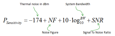
Sensitivity estimate in dBm. Each term adds to the noise floor or to the SNR the demodulator needs above it.

• -174 is labelled Thermal noise in dBm. It is the thermal noise power in 1 Hz at 290 K: 10 log₁₀(kT x 1000) = -173.98 dBm/Hz, rounded to -174.
• NF is labelled Noise Figure. It is how much the receiver raises the noise above the thermal level, in dB.
• The bandwidth term is 10 log₁₀(BW), with BW in Hz. The drawing places BW like an exponent of log₁₀, but it is the argument of the log.
• SNR is labelled Signal To Noise Ratio. It is the SNR the demodulator needs to meet the error rate criteria, in dB.

Let's put numbers into it for a 10 MHz LTE carrier. The occupied bandwidth is 50 RB x 180 kHz = 9 MHz, so the bandwidth term is 10 log₁₀(9 x 10⁶) = 69.5 dB. Assume a UE noise figure of 9 dB. Also assume the robust QPSK reference channel needs an SNR of about -1 dB. The estimate is then -174 + 9 + 69.5 - 1 = -96.5 dBm. For comparison, 36.101 Table 7.3.1-1 sets -97 dBm for Band 1 at 10 MHz. The NF and the SNR here are assumptions, so treat the closeness as a check of the method rather than a derivation of the requirement.

The bandwidth term can be checked directly against 36.101 Table 7.3.1-1. For Band 1 the requirement is -100 dBm at 5 MHz, -97 dBm at 10 MHz, -95.2 dBm at 15 MHz and -94 dBm at 20 MHz. Each doubling of the bandwidth costs 3 dB, and 10 log₁₀(75/50) = 1.76 dB explains the 15 MHz value. So the requirement follows the 10 log₁₀(BW) term exactly, while NF and SNR stay the same across bandwidths.

There are several major factors that influence on Sensitivity as listed below. The effect of the item i),ii),iii) can be seen in the equation shown above. In recent high end communication technology (e.g, WCDMA, LTE etc), many of techniques are added to improve sensitivity (i.e, decrease error rate and increase communication reliability). Most common techniques adopted in those high end communication are Adaptive Modulation and Channel Coding/Error Correction. As a result, item iv) and v) became an important factors for Sensitivity performance.

i) System Bandwidth

ii) Noise Figure

iii) SNR

iv) Modulation Scheme

v) Channel Coding / Error Correction Method

One of the examples showing the impact of item iii), iv), v) is shown below (Ref [1]). As you see, this graph does not directly show about Sensitivity, but the Sensitivity is directly related to BER or BLER. You may say High BLER indicate poor sensitivity performance and Low BLER indicate good sensitivity performance. This example is for LTE. The MCS value in LTE defines a specific modulation scheme and Code Rate (i.e, parameter of Channel Coding/Error Correction). As you see here, Low MCS shows lower BLER if SNR is same. It means Low MCS will show good sensitivity performance than higher MCS.

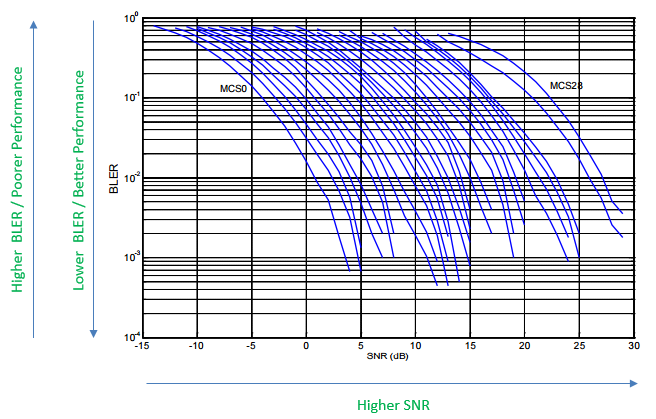
BLER versus SNR for LTE MCS0 to MCS28. A higher MCS needs a higher SNR for the same BLER.

• The horizontal axis is SNR from -15 dB to 30 dB. The vertical axis is BLER on a log scale from 10^-4 to 1.
• The leftmost curve is MCS0 and the rightmost is MCS28. At 10 % BLER the two curves are more than 25 dB apart.
• That spread in SNR moves the sensitivity by the same amount, because SNR adds to the formula dB for dB.

• Sensitivity is noise floor plus required SNR : the noise floor is -174 dBm/Hz + NF + 10 log₁₀(BW), and the demodulator sets the SNR.
• Doubling the bandwidth costs 3 dB : the 36.101 reference sensitivity for Band 1 falls from -100 dBm at 5 MHz to -94 dBm at 20 MHz for that reason.
• The SNR term depends on MCS : a robust MCS lowers the required SNR and so lowers the sensitivity number, which is why sensitivity tests use QPSK.
• 1 dB of NF is 1 dB of sensitivity : the LNA and everything in front of it sets the NF, so front end loss enters the sensitivity directly.

Conditions for Sensitivity Measurement

As mentioned above, there are many factors that influence the Sensitivity. So when you do sensitivity measurement, you have to clearly define the conditions for the measurement especially when you want to use the measured value for quality control or performance comparision with other devices. If you are working on well known/widely used communication system, the specific measurement conditions for Sensitity are defined in the industry standard /specification. For example, if you are working with Bluetooth, you may find those condition from Bluetooth SIG specification. If you are working on WLAN, you may find the condition from IEEE specification. In case of LTE, the conditions are defined in 3GPP 36.521.

Following is an example of Sensitivity measurement condition for LTE based on 3GPP 36.521 - 7.3 Reference sensitivity level.

The condition is specified as in 36.521-Table A.3.2-1. If I summarize the highlights, it is as follows

• No Interference (very good SNR)
• Number of RB : Maximum Number of RBs allowed for the specified System Bandwidth
• MCS : 4  // Sensitivity is measured with very robust demodulate condition.

LTE does not use BER as the criteria. 36.101 clause 7.3 defines REFSENS as the minimum mean power at each UE antenna port at which the throughput is at least 95 % of the maximum throughput of the reference measurement channel. The requirement assumes two Rx ports as the baseline, and both ports are tested at the same time. The UE uplink has to transmit during the test, and Table 7.3.1-2 limits its RB allocation so that the UE's own transmitter does not set the result.

The expected sensitity power (passing critieria) is defined in 36.521 - Table 7.3.5-1 for 2 Rx antenna case and Table 7.3_1.5-1 for 4 Rx antenna case. As you see, the passing criteria is slightly different for each system Bandwidth and with operating band(carrier frequency).

The test document is 36.521-1, and its numbers come from the 36.101 minimum requirement. The test requirement is 0.7 dB higher than the 36.101 value for every entry in the tables below. For example, Band 1 at 10 MHz is -97 dBm in 36.101 Table 7.3.1-1 and -96.3 dBm in 36.521-1 Table 7.3.5-1. The 0.7 dB is the test tolerance. It covers the uncertainty of the test equipment. For 4 Rx ports, 36.101 Table 7.3.1-1a lowers the requirement by 2.7 dB for bands such as 1, 2, 3, 7 and 20. So Band 2 at 5 MHz becomes -98 - 2.7 + 0.7 = -100.0 dBm in the 4 Rx table.

< 36.521 - Table A.3.2-1: Fixed Reference Channel for Receiver Requirements (FDD) >

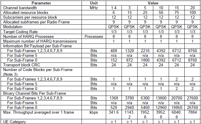
• The allocation is the full bandwidth: 6, 15, 25, 50, 75 and 100 RB for 1.4, 3, 5, 10, 15 and 20 MHz.
• The modulation is QPSK and the target coding rate is 1/3 for every bandwidth. There is one HARQ transmission, so no retransmission helps the result.
• Sub-frame 5 carries no allocation, shown as n/a. Sub-frame 0 carries a smaller payload at the narrow bandwidths, because PBCH and the synchronization signals take part of it. The maximum throughput at 10 MHz is 9 x 4392 bits per 10 ms = 3952.8 kbps.

< 36.521 - Table 7.3.5-1: Reference sensitivity QPSK P_PREFSENS >

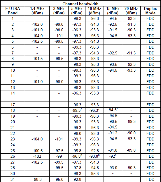
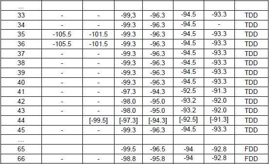
• Each row is an E-UTRA band, and each column is a channel bandwidth. Across a row the value rises by about 3 dB per doubling of bandwidth.
• Down a column the value changes with the band. For example, Band 1 at 10 MHz is -96.3 dBm and Band 3 at 10 MHz is -93.3 dBm.
• Values in square brackets, as for Band 44, were not yet final in the version captured here.

< 36.521 - Table 7.3_1.5-1: Reference sensitivity QPSK P_PREFSENS >

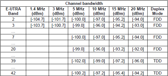
• Only the bands that allow 4 Rx ports appear. Every value is in square brackets in this capture.
• Band 2 at 5 MHz is [-100.0] dBm, 2.7 dB lower than the -97.3 dBm of the 2 Rx table. The 2.7 dB is the 36.101 ΔR_IB,4R value for that band.

• A sensitivity number is only meaningful with its conditions : bandwidth, RB allocation, MCS, Rx port count and the pass criteria all move it by several dB.
• LTE measures throughput, not BER : REFSENS is the lowest power at which the reference channel still reaches 95 % of its maximum throughput.
• 36.521-1 adds the test tolerance to 36.101 : the conformance value is 0.7 dB above the minimum requirement.
• More Rx ports give a stricter requirement : 4 Rx ports lower the requirement by 2.7 dB in the listed bands, which is close to the 3 dB of doubling the collected power.

Reference

[1] NISTIR 7986 - LTE Physical Layer Performance Analysis by Wen-Bin Yang, Michael Souryal

[2] 3GPP TS 36.101 v20.0.0 - E-UTRA UE radio transmission and reception, clause 7.3 and Table 7.3.1-1