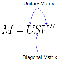
Singluar Value Decomposition is a technique which decompose a matrix into three components as follows. The diagonal indicate the singular values and the Unitary Matrix parts indicates the basis of each components. Depending on the nature of the original matrix M, you can interprete the U, V, S in many different ways. (Check Unitary Matrix page if you are not familiar with the concept and property of this matrix)
- What do U, S and V mean ?
- Geometrical Interpretation of SVD
- How do you calculate the SVD by hand ?
- Applications
- Reference
What do U, S and V mean ?
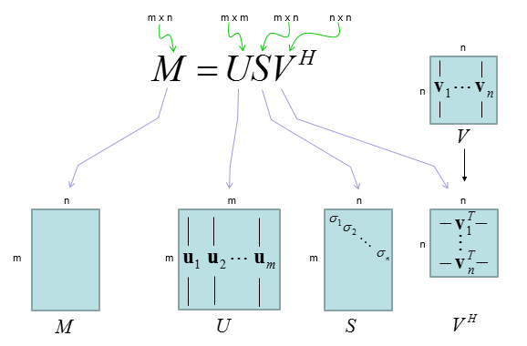
Before we look at any geometry, let's fix what each factor is. For an m x n matrix M, U is m x m, S is m x n and V is n x n. The diagrams below show where each factor comes from and what it does to a vector.
If we do some dimension analysis and look into the meaning of each component matrix, it can be illustrated as follows.
(Look into Orthonormal matrix and Eigenvector page if you are not familiar with the concept and property of those matrix)
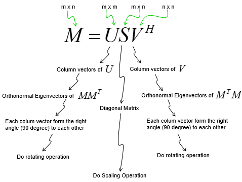
This technique has various applications like PCA (Principal Component Analysis) in Statistics and MIMO channel analysis in radio communications and solving a linear system equation (linear Matrix equation) etc. (I put the link for some of the YouTube video showing the applications of SVD in Reference Section).
With this, we can decompose a matrix into three matrices that perform following three transformation in sequence. (SVD is tightly related to PCA (Principal Component Analysis))
- a first rotation in the input space
- a simple positive scaling that takes a vector in the input space to the output space
- another rotation in the output space
If you look into each matrix and meaning of matrix elements, it can be illustrated as follows. Each u vectors are orthogonal to each other and each v vectors are orthogonal to each other.
NOTE :
- u1,u2,..,um is orthogonal to each other. It means if you draw the vector in cartesian coordinate they form right angle (90 degree) to each other.
- v1,v2,..,vn is orthogonal to each other. It means if you draw the vector in cartesian coordinate they form right angle (90 degree) to each other.
The two diagrams above leave out one precise statement, so let's add it. The columns of V are eigenvectors of MHM, and the columns of U are eigenvectors of MMH. Both products have the same nonzero eigenvalues, and the singular values are their square roots. The singular values sit on the diagonal of S in decreasing order, σ1 >= σ2 >= ... >= 0.
Singular values are not eigenvalues of M : they are the square roots of the eigenvalues of MHM. The two sets agree only when M is Hermitian positive semidefinite, for example a covariance matrix.The rank is the number of nonzero singular values : an m x n matrix of rank r has exactly r positive values of σ, and the rest of the diagonal of S is zero.A rotation here can include a reflection : U and V are unitary, so they keep lengths and angles. A real orthogonal matrix with determinant -1 is a reflection, and two of the examples below contain one.The scaling is nonnegative, not always positive : a singular value can be 0. Then S removes that direction completely, and M loses rank.
Geometrical Interpretation of SVD
I will try to represent the properties (each steps) of SVD in geometric form to help you to get some intuitive understanding. But understanding the meaning of the graphical representation itself may not always be easy and sometimes would confuse you even further. Just try to look into each of the plots and try to correlate the graph to the mathematical representation shown above. I hope there can be a way to get you understand this concept just by looking at something.. but unfortunately there is no such a thing in learning anything. You just get small pieces of help from here and there and gradually build up your own intuition. I hope this section can give you at least some help rather than total confusion :)
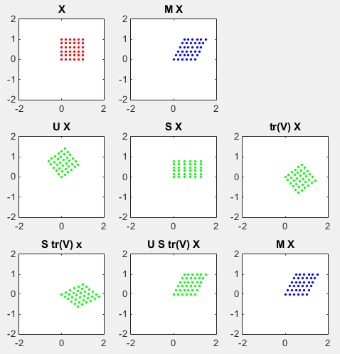
As you recall from the early part of this page, a matrix can magnify or rotate or shear the set of dots(points in a coordinate). SVD is a method to convert the whole transformational process into each separate transformation component, that is, rotational component, magnifying component and another rotational component. A graphical presentation of SVD is as follows. (I also posted the Octave/Matlab script that I wrote for this illustration and play with various other matrix('tm' in the script) and see the result until get some intuitive feeling about this process).
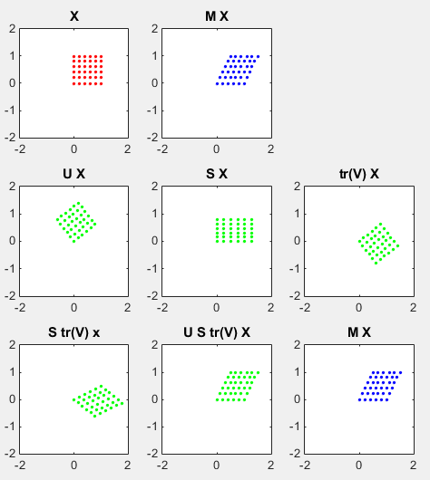
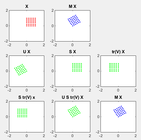
There are many different ways to visualize SVD operation. Following is the way I visualize the SVD operation. The intention to this illustration is to show how each componet of SVD transform the orignal data(input). It may not make sense to you right away, but give you some time to think of each of the plot with the description below, it will (hopefully) gradually make sense.
(1) : this is the set of input vectors (each red dot indicate a vector) that will be transformed by the matrix M
(2) : this shows the result of the transformation performed by the matrix M
(3) : this shows the transformation done by U component of SVD. Here, you see that U perform rotation operation only. It does not do any scaling. It does not do any shearing.
(4) : this shows the transformation done by S component of SVD. Here, you see that S perform scaling operation only. It does not do any rotation. It does not do any shearing
(5) : this shows the transformation done by VH( or transpose(V)) component of SVD. Here, you see that VH perform rotation operation only. It does not do any scaling. It does not do any shearing
(8) : Same as (5)
(7) : Shows the transformation that step (5) and step (4) do together
(6) : Shows the transformation that step (5), step (4) and step (3) do together. This is same as the transformation that M matrix does.
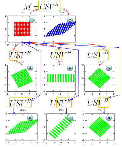
Two pairs of panels must match : panel 6 applies U S VH, which is M itself, so it matches panel 2. Panel 8 applies VH alone again, so it matches panel 5.S never turns the grid : S is diagonal, so it stretches or shrinks along the x and y axes only. The rows and columns of dots in panel 4 stay horizontal and vertical.The shear comes from the combination : U and VH keep the grid square, and S keeps it rectangular. Only the rotation, the unequal stretch and the second rotation together produce the slanted shape of panel 2.The code below uses a smaller grid : the grid in the diagram above runs from -1 to 1. The listing below uses dots from 0 to 1, so its plots show one corner of that grid.
I put some more examples with matlab code for practice. try to interpret each of the plots yourself.
Look at the graphs on the top row. The red dots on left graph are transformed by the matrix M to be the blue dots on right graph.
Look at the graph on the middle row. The dots on left graph is the result of transforming X with the matrix U. You can see here that the area of the original rectangle(array of red dots) does not changes, but it get rotated. The dots on the graph in the middle is the result of transforming X with the matrix S. You don't see any rotation here, but you see the original rectangle (array of red dots) get extended in x direction and contracted in y direction. The dots on right graph is the result of transforming X with the matrix V*(V Hermitian). You can see here that the area of the original rectangle(array of red dots) does not changes, but it get rotated.
clear all;

ptList_x=[];
ptList_y=[];

for y=0.0:0.2:1.0
for x=0.0:0.2:1.0
    ptList_x=[ptList_x x];
    ptList_y=[ptList_y y];
end
end

ptList_v = [ptList_x' ptList_y'];
ptList_v = ptList_v';

%tm = [1.25 1;0.2 0.9]
%tm = [1.0 0.5;0.0 1.0]
%tm = [1.2 0.0;0.0 1.5]
%tm = [cos(pi/6) -sin(pi/6);sin(pi/6) cos(pi/6)]
tm = [1.0 0.5;0.0 1.0]

[U,S,V]=svd(tm)

ptList_v_tm = tm * ptList_v;
ptList_v_tm_x = ptList_v_tm(1,:);
ptList_v_tm_x = ptList_v_tm_x';
ptList_v_tm_y = ptList_v_tm(2,:);
ptList_v_tm_y = ptList_v_tm_y';

ptList_v_tm_u = U * ptList_v;
ptList_v_tm_u_x = ptList_v_tm_u(1,:);
ptList_v_tm_u_x = ptList_v_tm_u_x';
ptList_v_tm_u_y = ptList_v_tm_u(2,:);
ptList_v_tm_u_y = ptList_v_tm_u_y';

ptList_v_tm_s = S * ptList_v;
ptList_v_tm_s_x = ptList_v_tm_s(1,:);
ptList_v_tm_s_x = ptList_v_tm_s_x';
ptList_v_tm_s_y = ptList_v_tm_s(2,:);
ptList_v_tm_s_y = ptList_v_tm_s_y';

ptList_v_tm_v = (conj(V)') * ptList_v;
ptList_v_tm_v_x = ptList_v_tm_v(1,:);
ptList_v_tm_v_x = ptList_v_tm_v_x';
ptList_v_tm_v_y = ptList_v_tm_v(2,:);
ptList_v_tm_v_y = ptList_v_tm_v_y';

ptList_v_tm_vs = S * (conj(V)') * ptList_v;
ptList_v_tm_vs_x = ptList_v_tm_vs(1,:);
ptList_v_tm_vs_x = ptList_v_tm_vs_x';

ptList_v_tm_vs_y = ptList_v_tm_vs(2,:);
ptList_v_tm_vs_y = ptList_v_tm_vs_y';

ptList_v_tm_usv = U * S * (conj(V)') * ptList_v;
ptList_v_tm_usv_x = ptList_v_tm_usv(1,:);
ptList_v_tm_usv_x = ptList_v_tm_usv_x';
ptList_v_tm_usv_y = ptList_v_tm_usv(2,:);
ptList_v_tm_usv_y = ptList_v_tm_usv_y';

subplot(3,3,1);
plot(ptList_x,ptList_y,'ro','MarkerFaceColor',[1 0 0],'MarkerSize',2.0);
axis([-2 2 -2 2]);title('X');

subplot(3,3,2);
plot(ptList_v_tm_x,ptList_v_tm_y,'bo','MarkerFaceColor',[0 0 1],'MarkerSize',2.0);
axis([-2 2 -2 2]);title('M X');

subplot(3,3,4);
plot(ptList_v_tm_u_x,ptList_v_tm_u_y,'go','MarkerFaceColor',[0 1 0],'MarkerSize',2.0);
axis([-2 2 -2 2]);title('U X');

subplot(3,3,5);
plot(ptList_v_tm_s_x,ptList_v_tm_s_y,'go','MarkerFaceColor',[0 1 0],'MarkerSize',2.0);
axis([-2 2 -2 2]);title('S X');

subplot(3,3,6);
plot(ptList_v_tm_v_x,ptList_v_tm_v_y,'go','MarkerFaceColor',[0 1 0],'MarkerSize',2.0);
axis([-2 2 -2 2]);title('tr(V) X');

subplot(3,3,7);
plot(ptList_v_tm_vs_x,ptList_v_tm_vs_y,'go','MarkerFaceColor',[0 1 0],'MarkerSize',2.0);
axis([-2 2 -2 2]);title('S tr(V) x');

subplot(3,3,8);
plot(ptList_v_tm_usv_x,ptList_v_tm_usv_y,'go','MarkerFaceColor',[0 1 0],'MarkerSize',2.0);
axis([-2 2 -2 2]);title('U S tr(V) X');

subplot(3,3,9);
plot(ptList_v_tm_x,ptList_v_tm_y,'bo','MarkerFaceColor',[0 0 1],'MarkerSize',2.0);
axis([-2 2 -2 2]);title('M X');
A second view with column vectors
The dot plots show the effect on many points at once. A cleaner view follows only the two columns of each matrix, because a 2 x 2 matrix is fully defined by where it sends (1, 0) and (0, 1).
I will try another type of graphical representation as follows. (Red arrow indicates the first column vector of a matrix and blue arrow indicates the second column vector of a matrix. tr(V) means " V', V transpose")
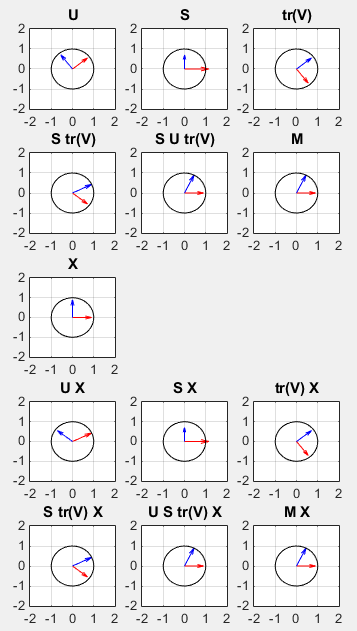
Following is the Matlab Code for this representation. I know it is too long and messy, but I think it would be easier to read. Just try change 'M' or 'X' matrix and see what you get and try to interpret the result. The black circle is a circle with the radius 1 to help you to estimate the magnitue of each vector.
clear all;
M = [1.0 0.5;0.0 1.0]
[U,S,V]=svd(M)

SV = S*V'
USV = U*S*V'

u1 = U(:,1);
u2 = U(:,2);
s1 = S(:,1);
s2 = S(:,2);
vT = V';
vT1 = vT(:,1);
vT2 = vT(:,2);

sv1 = SV(:,1);
sv2 = SV(:,2);
usv1 = USV(:,1);
usv2 = USV(:,2);
m1 = M(:,1)';
m2 = M(:,2)';

X = [1 0;0 1];
x1 = X(:,1);
x2 = X(:,2);

X_VT = V' * X;
x_vT1 = X_VT(:,1);
x_vT2 = X_VT(:,2);

X_S = S * X;
x_s1 = X_S(:,1);
x_s2 = X_S(:,2);

X_U = S * U;
x_u1 = X_U(:,1);
x_u2 = X_U(:,2);

x_sv1 = SV(:,1);
x_sv2 = SV(:,2);

x_usv1 = USV(:,1);
x_usv2 = USV(:,2);

x_m1 = M(:,1);
x_m2 = M(:,2);

t = linspace(0,2*pi,50);

% plot the first row
subplot(5,3,1);
quiver(0,0,u1(1),u1(2),'r','MaxHeadSize',1.5);
axis([-2 2 -2 2]);
hold on;
quiver(0,0,u2(1),u2(2),'b','MaxHeadSize',1.5);
axis([-2 2 -2 2]);
title('U');
hold on;
plot(cos(t),sin(t),'k-');
set(gca,'xtick',[-2 -1 0 1 2]);set(gca,'ytick',[-2 -1 0 1 2]);
grid();
hold off;

subplot(5,3,2);
quiver(0,0,s1(1),s1(2),'r','MaxHeadSize',1.5);
axis([-2 2 -2 2]);
hold on;
quiver(0,0,s2(1),s2(2),'b','MaxHeadSize',1.5);
axis([-2 2 -2 2]);
title('S');
hold on;
plot(cos(t),sin(t),'k-');
set(gca,'xtick',[-2 -1 0 1 2]);set(gca,'ytick',[-2 -1 0 1 2]);
grid();
hold off;

subplot(5,3,3);
quiver(0,0,vT1(1),vT1(2),'r','MaxHeadSize',1.5);
axis([-2 2 -2 2]);
hold on;
quiver(0,0,vT2(1),vT2(2),'b','MaxHeadSize',1.5);
axis([-2 2 -2 2]);
title('tr(V)');
hold on;
plot(cos(t),sin(t),'k-');
set(gca,'xtick',[-2 -1 0 1 2]);set(gca,'ytick',[-2 -1 0 1 2]);
grid();
hold off;

% plot the second row
subplot(5,3,4);
quiver(0,0,sv1(1),sv1(2),'r','MaxHeadSize',1.5);
axis([-2 2 -2 2]);
hold on;
quiver(0,0,sv2(1),sv2(2),'b','MaxHeadSize',1.5);
axis([-2 2 -2 2]);
title('S tr(V)');
hold on;
plot(cos(t),sin(t),'k-');
set(gca,'xtick',[-2 -1 0 1 2]);set(gca,'ytick',[-2 -1 0 1 2]);
grid();
hold off;

subplot(5,3,5);
quiver(0,0,usv1(1),usv1(2),'r','MaxHeadSize',1.5);
axis([-2 2 -2 2]);
hold on;
quiver(0,0,usv2(1),usv2(2),'b','MaxHeadSize',1.5);
axis([-2 2 -2 2]);
title('S U tr(V)');
hold on;
plot(cos(t),sin(t),'k-');
set(gca,'xtick',[-2 -1 0 1 2]);set(gca,'ytick',[-2 -1 0 1 2]);
grid();
hold off;

subplot(5,3,6);
quiver(0,0,m1(1),m1(2),'r','MaxHeadSize',1.5);
axis([-2 2 -2 2]);
hold on;
quiver(0,0,m2(1),m2(2),'b','MaxHeadSize',1.5);
axis([-2 2 -2 2]);
title('M');
hold on;
plot(cos(t),sin(t),'k-');
set(gca,'xtick',[-2 -1 0 1 2]);set(gca,'ytick',[-2 -1 0 1 2]);
grid();
hold off;

% plot the third row
subplot(5,3,7);
quiver(0,0,x1(1),x1(2),'r','MaxHeadSize',1.5);
axis([-2 2 -2 2]);
hold on;
quiver(0,0,x2(1),x2(2),'b','MaxHeadSize',1.5);
axis([-2 2 -2 2]);
title('X');
hold on;
plot(cos(t),sin(t),'k-');
set(gca,'xtick',[-2 -1 0 1 2]);set(gca,'ytick',[-2 -1 0 1 2]);
grid();
hold off;

% plot the forth row
subplot(5,3,10);
quiver(0,0,x_u1(1),x_u1(2),'r','MaxHeadSize',1.5);
axis([-2 2 -2 2]);
hold on;
quiver(0,0,x_u2(1),x_u2(2),'b','MaxHeadSize',1.5);
axis([-2 2 -2 2]);
title('U X');
hold on;
plot(cos(t),sin(t),'k-');
set(gca,'xtick',[-2 -1 0 1 2]);set(gca,'ytick',[-2 -1 0 1 2]);
grid();
hold off;

subplot(5,3,11);
quiver(0,0,x_s1(1),x_s1(2),'r','MaxHeadSize',1.5);
axis([-2 2 -2 2]);
hold on;
quiver(0,0,x_s2(1),x_s2(2),'b','MaxHeadSize',1.5);
axis([-2 2 -2 2]);
title('S X');
hold on;
plot(cos(t),sin(t),'k-');
set(gca,'xtick',[-2 -1 0 1 2]);set(gca,'ytick',[-2 -1 0 1 2]);
grid();
hold off;

subplot(5,3,12);
quiver(0,0,x_vT1(1),x_vT1(2),'r','MaxHeadSize',1.5);
axis([-2 2 -2 2]);
hold on;
quiver(0,0,x_vT2(1),x_vT2(2),'b','MaxHeadSize',1.5);
axis([-2 2 -2 2]);
title('tr(V) X');
hold on;
plot(cos(t),sin(t),'k-');
set(gca,'xtick',[-2 -1 0 1 2]);set(gca,'ytick',[-2 -1 0 1 2]);
grid();
hold off;

% plot the fifth row
subplot(5,3,13);
quiver(0,0,x_sv1(1),x_sv1(2),'r','MaxHeadSize',1.5);
axis([-2 2 -2 2]);
hold on;
quiver(0,0,x_sv2(1),x_sv2(2),'b','MaxHeadSize',1.5);
axis([-2 2 -2 2]);
title('S tr(V) X');
hold on;
plot(cos(t),sin(t),'k-');
set(gca,'xtick',[-2 -1 0 1 2]);set(gca,'ytick',[-2 -1 0 1 2]);
grid();
hold off;

subplot(5,3,14);
quiver(0,0,x_usv1(1),x_usv1(2),'r','MaxHeadSize',1.5);
axis([-2 2 -2 2]);
hold on;
quiver(0,0,x_usv2(1),x_usv2(2),'b','MaxHeadSize',1.5);
axis([-2 2 -2 2]);
title('U S tr(V) X');
hold on;
plot(cos(t),sin(t),'k-');
set(gca,'xtick',[-2 -1 0 1 2]);set(gca,'ytick',[-2 -1 0 1 2]);
grid();
hold off;

subplot(5,3,15);
quiver(0,0,x_m1(1),x_m1(2),'r','MaxHeadSize',1.5);
axis([-2 2 -2 2]);
hold on;
quiver(0,0,x_m2(1),x_m2(2),'b','MaxHeadSize',1.5);
axis([-2 2 -2 2]);
title('M X');
hold on;
plot(cos(t),sin(t),'k-');
set(gca,'xtick',[-2 -1 0 1 2]);set(gca,'ytick',[-2 -1 0 1 2]);
grid();
hold off;
Two lines in this listing do not match their titles, and the plot above shows the effect. The line X_U = S * U computes S U, not U X, so the panel titled 'U X' shows the columns of S U. For this M, those columns are (1.0095, 0.4805) and (-0.7882, 0.6154), and they are the arrows in that panel. The line X_U = U * X would repeat the U panel of the first row, because X is the identity matrix. Also, the title 'S U tr(V)' in the second row should read 'U S tr(V)', because the listing computes USV = U*S*V'.
Let's look into some examples shown below. I will show you both types of graphical representation for the same matrix.
Example 1 - a diagonal matrix
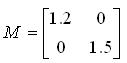
The first matrix, M = [1.2 0 ; 0 1.5], only scales. It stretches x by 1.2 and y by 1.5, and it has no rotation or shear. So you may expect U and V to be identity matrices. They are not, and the reason is the ordering rule of SVD.
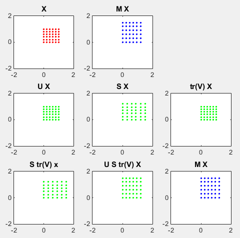
Look at the graphs on the top row. The red dots on left graph are transformed by the matrix M to be the blue dots on right graph.
Look at the graph on the middle row. The dots on left graph is the result of transforming X with the matrix U. You can see here that the area of the original rectangle(array of red dots) does not changes, and it does not get rotated either(it means that the matrix M does not have any rotational property). The dots on the graph in the middle is the result of transforming X with the matrix S. You don't see any rotation here, but you see the original rectangle (array of red dots) get extended in both x and y direction. The dots on right graph is the result of transforming X with the matrix V*(V Hermitian). You can see here that the area of the original rectangle(array of red dots) does not changes, and it does not get rotated either(it means that the matrix M does not have any rotational property).
Followings are each component matrix of the SVD decomposition calculated with Matlab. Look at each matrix and see if you can visualize the properties of each matrix in your brain. For this reason (for visualizing the matrix in your brain without much calculation), I picked simple 2 x 2 matrix (If you need some practice, refer to Matrix : Transformation page).
|
U |
S |
V |
|
0 1 1 0 |
1.5000 0 0 1.2000 |
0 1 1 0 |
Following is the result of applying each of these matrix component to an 2 dimensional array of points to help you visualize and understand the meaning of these matrix more intuitively.
Following is another type of presentation. See if you can correlate this with the one above.
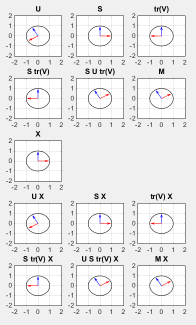
The column vector picture above repeats the one for Example 2. Its U panel shows the vectors (-0.866, -0.5) and (-0.5, 0.866), which are the columns of U in Example 2. For this diagonal matrix, the U and tr(V) panels would show the swapped unit vectors (0, 1) and (1, 0), and the S panel would show (1.5, 0) and (0, 1.2).
SVD sorts the singular values : S = [1.5 0 ; 0 1.2] lists the larger stretch first. In M the larger stretch is on the y axis, so U and V must swap x and y.U and V here are reflections : [0 1 ; 1 0] has determinant -1, and it mirrors the plane across the line y = x. The grid of dots is symmetric about that line, so the U X and tr(V) X plots look unchanged.The two swaps cancel : U S VT = [1.2 0 ; 0 1.5], so the product gives M back.
Example 2 - a rotation matrix
The second matrix is a pure rotation by 30 degrees, π/6. A rotation keeps every length, so both of its singular values must be 1. The interesting part is how SVD splits one rotation between U and V.
Try interpret the following example as described in above example.
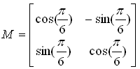
Followings are each component matrix of the SVD decomposition calculated with Matlab. Look at each matrix and see if you can visualize the properties of each matrix in your brain. For this reason (for visualizing the matrix in your brain without much calculation), I picked simple 2 x 2 matrix (If you need some practice, refer to Matrix : Transformation page).
|
U |
S |
V |
|
-0.8660 -0.5000 -0.5000 0.8660 |
1 0 0 1 |
-1 0 0 1 |
Following is the result of applying each of these matrix component to an 2 dimensional array of points to help you visualize and understand the meaning of these matrix more intuitively.
Following is another type of presentation. See if you can correlate this with the one above.
S is the identity : both singular values are 1, so the S X plot is the unchanged grid. U and V do all of the work.Two reflections make one rotation : U = [-0.866 -0.5 ; -0.5 0.866] and V = [-1 0 ; 0 1] both have determinant -1, so each one is a reflection. Their product U VT = [0.866 -0.5 ; 0.5 0.866] is the 30 degree rotation.The SVD of a rotation is not unique : when all singular values are equal, any orthogonal V works together with U = M V. Matlab returned one choice. U = M together with the identity matrix as V would be equally correct.
Example 3 - a shear matrix
The third matrix is the shear [1 0.5 ; 0 1] used in the listings above. Both of its eigenvalues are 1, yet it changes lengths, so its singular values cannot both be 1. The next section computes them by hand.
Try interpret the following example as described in above example.
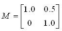
Followings are each component matrix of the SVD decomposition calculated with Matlab. Look at each matrix and see if you can visualize the properties of each matrix in your brain. For this reason (for visualizing the matrix in your brain without much calculation), I picked simple 2 x 2 matrix (If you need some practice, refer to Matrix : Transformation page).
|
U |
S |
V |
|
0.7882 -0.6154 0.6154 0.7882 |
1.2808 0 0 0.7808 |
0.6154 -0.7882 0.7882 0.6154 |
Following is the result of applying each of these matrix component to an 2 dimensional array of points to help you visualize and understand the meaning of these matrix more intuitively.
Following is another type of presentation. See if you can correlate this with the one above.
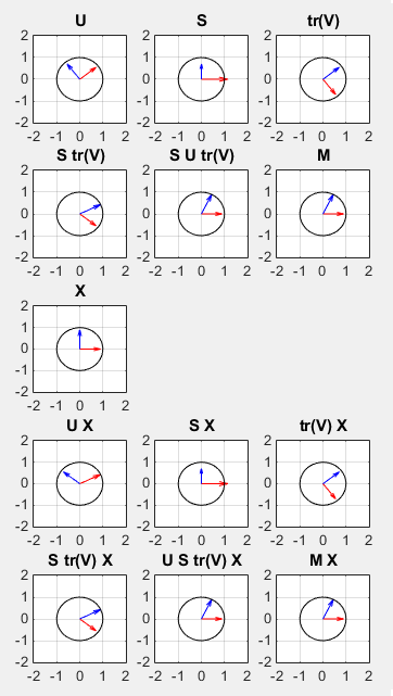
Eigenvalues and singular values differ : M is triangular with 1 on the diagonal, so both eigenvalues are 1. The singular values are 1.2808 and 0.7808, because M is not symmetric.Area is preserved : 1.2808 x 0.7808 = 1.0000 = det(M). The stretch along one axis is exactly undone by the shrink along the other.U and V are true rotations here : both have determinant +1. U turns by 38.0 degrees and V by 52.0 degrees, and the next section shows where these angles come from.
How do you calculate the SVD by hand ?
The plots above show what U, S and V do. Now let's compute them for the shear matrix of Example 3, so you can see where each number in its table comes from. The method needs only the eigen decomposition of MTM and one matrix multiplication.
M = [ 1  0.5 ; 0  1 ]

step 1   MTM = [ 1  0.5 ; 0.5  1.25 ]
         det( MTM - λ I ) = λ2 - 2.25 λ + 1 = 0
         λ1 = 1.6404       λ2 = 0.6096

step 2   σ1 = √1.6404 = 1.2808       σ2 = √0.6096 = 0.7808

step 3   eigenvectors of MTM
         v1 = ( 0.6154, 0.7882 )       v2 = ( -0.7882, 0.6154 )

step 4   u1 = M v1 / σ1 = ( 1.0095, 0.7882 ) / 1.2808 = ( 0.7882, 0.6154 )
         u2 = M v2 / σ2 = ( -0.4805, 0.6154 ) / 0.7808 = ( -0.6154, 0.7882 )
These are exactly the values in the table of Example 3. The singular values also have a closed form here, σ = (√17 + 1)/4 and (√17 - 1)/4. So their product is 1, which is det(M), and their difference is 0.5, the shear factor.
Step 4 is the SVD written one column at a time. If you multiply M = U S VT on the right by V, you get M V = U S, and column i of that equation is M vi = σi ui. Computing ui this way also keeps the signs of ui and vi consistent. If you took the eigenvectors of MMT separately, a sign could come out wrong, and U S VT would no longer give M.
The angles tell the geometric story. V is a rotation by 52.0 degrees, so VT first turns the input by -52.0 degrees. S then stretches the new x axis by 1.2808 and shrinks the new y axis to 0.7808. Finally U turns the result by 38.0 degrees. That is the middle row of the dot plot for this matrix.
Use MTM for V and M vi for U : the eigenvectors of MTM give V, and ui = M vi / σi gives U with matching signs.A zero singular value needs another rule : if σi = 0, the division in step 4 fails. Then ui is any unit vector orthogonal to the other columns of U.Software does not form MTM : forming MTM squares the condition number and loses small singular values. LAPACK and Matlab reduce M to a bidiagonal matrix with Householder reflections and then iterate on that.
Applications
Why is SVD worth this much effort? The singular values sort a matrix into pieces by importance, from the largest σ to the smallest. Each application below uses that ordering in a different way.
All three applications use the outer product form of the SVD, M = σ1 u1 v1H + σ2 u2 v2H + ... . If you keep only the first k terms, you get the best rank k approximation of M. This result is the Eckart-Young theorem. The error of that approximation, in the Frobenius norm, is the square root of the sum of the squares of the dropped singular values. For the shear matrix above, the rank 1 approximation is below, and its error is exactly σ2 = 0.7808.
σ1 u1 v1T = 1.2808 x ( 0.7882 ; 0.6154 ) ( 0.6154  0.7882 ) = [ 0.6213  0.7957 ; 0.4851  0.6213 ]

|| M - σ1 u1 v1T ||F = 0.7808 = σ2
The same singular values answer several other questions. The rank of M is the number of nonzero σ, and the condition number is σ1 / σn. The pseudo-inverse M+ = V S+ UH inverts each nonzero σ and solves least squares problems even when M loses rank. In a MIMO channel H = U S VH, the transmitter precodes with V and the receiver multiplies by UH. The channel then becomes parallel streams, and their gains are the singular values.
Truncation is optimal : no rank k matrix is closer to M than the first k terms of its SVD. This is why PCA and image compression keep the largest singular values.The dropped singular values are the error : you can read the approximation error from S before computing anything else.Small singular values amplify noise : the pseudo-inverse divides by each σ. So a very small σ is often set to zero on purpose, which is called truncated SVD.
Reference
- 1976 Matrix Singular Value Decomposition Film (YouTube)
- PCA, SVD (YouTube)
- Singular Value Decomposition, Linear Algebra - Detailed explanation of a worked example (YouTube)