Affine Mapping is an area of applying Matrix to geomatric transformation. This is a linear transformation followed by an optional translation (the same transform is applied to every points of the object being transformed).

Computer graphics, robotics and image processing all use this mapping. In each case every point p of an object moves to p' = Tp + t, where T is a matrix and t is a vector. When t = 0, the mapping is linear. When t is not zero, the origin itself moves, so the mapping is affine but not linear. I'll start with pictures of what a 2 x 2 matrix does to a shape. Then we'll write the math without and with translation, and finish with the order of operations and the properties an affine map keeps.

• Intuitive Meaning
• Transformation without translation
• Identity
• Scaling
• Shear
• Rotation
• Transformation with translation
• Why does the order of transformations matter ?
• What does an affine map keep and what does it change ?
• Example - Translation in 3D
• Example - Rotation in 3D
• Example - Rotation and Translation

Intuitive Meaning

Let's take an intuive approach first. Before any formula, it helps to see what a matrix does to a picture. A 2 x 2 matrix can stretch, flip, slant or turn a flat shape. The pictures below show each of these effects on the letter M.

My own image for a matrix is a kind of machine that is doing things as follows. As you see in the illustration, Matrix is taking in a shape (geometrical shape/object) and transform (change shape) them in mainly four different way as follows.

i) Scale (magnify or shrink)

ii) Rotate

iii) Shear(Skew)

iv) Reflection

In reality, a matrix can do more than one type of transformation like "Scale and Skew", "Scale and Rotate and Skew" etc.

I will talk about this kind of transformation in this section and I hope you can have some intuitive understanding of the propery of a matrix since it can be visualized as in this section.

The illustration below draws this idea as a machine. A square goes in at the top and passes through three blocks, Expand/Contract, Rotate and Shear. The shapes that come out at the bottom are squares of other sizes, turned squares and parallelograms. Reflection, the fourth item in the list, has no block of its own in the drawing. The examples below show it.

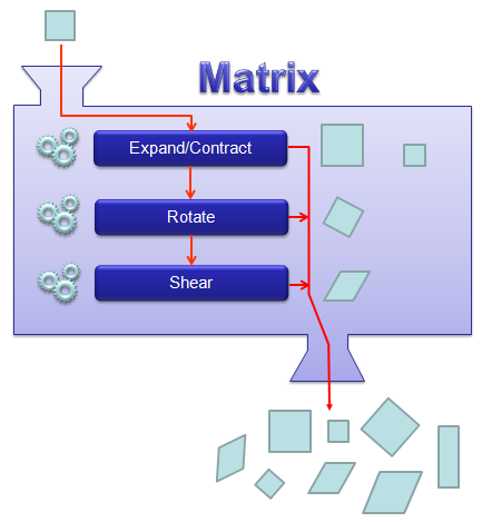
Figure 1. A matrix as a transformation machine. One matrix can scale, rotate and shear a shape, alone or in combination.

I think one of the best way to understand the characteristics of a Matrix is to apply it for an shape in a graphical coordinates and observe the result. Of course, there would be a certain limitation in this method since we can only visualize three dimensional shape and as a result the dimension of the matrix we can visualize would be 3 x 3 (or 4 x 4 in some cases). But if you build up a solid intuitive understanding of a properties of a matrix in this way, you can easily extend the understanding to any size of the matrix and, more importantly, you can understand more easily a mathematical model represented in the matrix format.

I will use a shape in two dimensional coordinate and 2 x 2 matrix applying to the shape on the coordinate. Here you see coordinates labeled (x1,y1) and (x2,y2). (x1,y1) represents each points before it is transformed by the matrix and (x2,y2) is the new points after (x1,y1) is transformed by the matrix.

Let's look at the first case. The first matrix is what we call Identity Matrix which has the value '1' in all the elements on diagonal line running from left top to right bottom and all the other elements are set to be '0'.

What is the result of the transformation of a shape transformed by the Identity Matrix ? The answer is "No change".

Figure 2. The identity matrix. Every point keeps its coordinates, so (x2,y2) = (x1,y1).

Next look at another matrix shown below. This matrix also looks similar to diagonal matrix but not exactly same. The difference is that the first element on the diagonal line is '-1' in stead of '1'.  What is the result ?

The shape is flipped around y axis.

Figure 3. Reflection about the y axis. The matrix changes the sign of x and keeps y.

Look at where the result is drawn. The matrix gives x2 = -x1 and y2 = y1, so every point moves to the other side of the y axis. The reflected grid should therefore sit in the second quadrant, to the left of the y axis. Figure 3 draws it in its original place instead. The circled point does show the flip correctly, because it moves from the left end of the M to the right end. Figure 4 and Figure 5 draw their results in the correct quadrant.

Next look at another matrix shown below. This matrix also looks similar to diagonal matrix but not exactly same. The difference is that the second element on the diagonal line is '-1' in stead of '1'.  What is the result ?

The shape is flipped around x axis.

Figure 4. Reflection about the x axis. The matrix changes the sign of y, so the M becomes a W below the x axis.

Next look at another matrix shown below. In this case, all the elements on the diagonal lines is set to be '-1' instead of '1'.  What is the result ?

It became reflected around the point (0,0). You can interpret this in two steps.

At the first step, the shape is flipped around y axis. and at the second step the shape is fliped around x axis.

Figure 5. Reflection through the origin. Both coordinates change sign, which is the same as a rotation by 180 degrees.

The two steps can be written as a product of the two matrices above. [[1, 0], [0, -1]] times [[-1, 0], [0, 1]] gives [[-1, 0], [0, -1]], where each inner bracket is one row. The order of the two steps does not matter here, because both matrices are diagonal.

Now let's look at another matrix as shown below. This time you see all '1's on the diagonal line and now you see a non-zero value out side of diagonal line. What is the result ?

The image shears.

Figure 6. Shear along x. Each point moves sideways by 0.3 times its height, so the square grid becomes a parallelogram.

The matrix in Figure 6 is [[1.0, 0.3], [0.0, 1.0]]. So x2 = x1 + 0.3 y1 and y2 = y1. Points on the x axis stay where they are, and points higher up move further to the right. For example, the point (0, 1) moves to (0.3, 1). The area of the grid does not change, because the determinant of the matrix is 1.

Now let's look at another matrix as shown below. This time you see the non-zero value in all the elements. This is tricky to analyze since these matrix can do almost everything described above.. but if the numbers in the elements can be represented as trigonometrix functions in the following format. This matrix can rotate the image as shown below.

Figure 7. Rotation by pi/4. Every point turns 45 degrees counterclockwise about the origin.

With θ = π/4, cos(θ) and sin(θ) are both 0.7071. So the point (1, 0) moves to (0.7071, 0.7071), and the point (1, 1) moves to (0, 1.4142). The distance of each point from the origin stays the same, which is why the grid keeps its square cells.

Actually this is only a few of the examples.. you can try any numbers in the matrix and apply to some shape and try to correlate those numbers to the result of the transformation until you build up your own intuition of figuring out the characteristics of a matrix.

Now let's do a little bit of math. But don't get scared .. it is not complicated. In some country, you would have learned this level of mathematics in high school. In some country, you would learn this in very early chapters of linear algebra. So in terms of calculation, this is very simple. Just focus on understanding the meaning of the math.

Transformation without translation

The first case is the one where we apply transformation only and no translation, meaning transformation without any shifting. It means the object will change only its shape but does not change the position. (Transformation means 'changing the shape' and translation means 'changing the position').

In this case, the mathematical expression for this can be represented as follows. Try to understand the meaning of each terms.

Figure 8. The transformation equation p' = Tp. The matrix T maps the original point p to the new point p'.

In case of transformation in 2 D plane, the equation can be represented as follows. Depending on what value you put as a,b,c,d, you can perform any transformation (scaling, shearing, rotation, reflection).

Figure 9. The 2D form. Four numbers a, b, c and d define the transformation.

In case of transformation in 3 D space, the equation can be represented as follows. Depending on what value you put as a,b,c,d,e,f,g,h,i, you can perform any transformation (scaling, shearing, rotation, reflection).

Figure 10. The 3D form. Nine numbers a to i define the transformation.

Written out, the 2D form says x' = ax + by and y' = cx + dy. Each new coordinate is a weighted sum of the old ones. So the first column [a, c]^T is where the point (1, 0) lands, and the second column [b, d]^T is where the point (0, 1) lands. This gives a quick way to build a matrix. Decide where the two unit vectors should go, and write them in as the columns.

Now the question is 'which value I have to plug into this matrix to achieve the transformation that I want'. Following shows the matrix for some basic transformation.

Identity

If you plug in numbers as shown below in 2D transform matrix, the object stay same (does not change the shape). The identity is the reference point for every other matrix in this list. Each of the others changes one or more of its entries, so compare them with this one.

Figure 11. The 2D identity matrix. Ones on the diagonal and zeros elsewhere.

If you plug in numbers as shown below in 3D transform matrix, the object stay same (does not change the shape)

Figure 12. The 3D identity matrix. Each coordinate is copied unchanged.

Scaling

If you plug in numbers as shown below in 2D transform matrix, you can magnify or shrink the shape. Depending on which value you put in Sx, Sy, the degree of scaling varies. Sx determines the scaling in x direction and Sy determines the scaling in y direction.

Figure 13. 2D scaling. S_x stretches x and S_y stretches y.

In 3D, the scaling matrix is defined as follows :

Figure 14. 3D scaling. A third factor S_z acts on z.

• A value above 1 magnifies, and a value between 0 and 1 shrinks : for example, S_x = 2 doubles every x coordinate.
• Equal factors keep the shape : when S_x = S_y, the object only changes size. Different factors stretch it more in one direction.
• A negative factor adds a reflection : S_x = -1 and S_y = 1 give the reflection of Figure 3.
• The determinant is the area factor : every area is multiplied by S_xS_y. In 3D, every volume is multiplied by S_xS_yS_z.

Note : If you want to see this transformation in more intuitive way, check these pages : scaling along X axis, scaling along Y axis, scaling along Z axis in www.slide4math.com

Shear

If you plug in numbers as shown below in 2D transform matrix, you can shear the object. The value of Sh determines the degree of shear. Shear slides each line of points along one axis, by an amount proportional to the other coordinate. Squares become parallelograms, but the area stays the same.

Figure 15. 2D shear. x' = x + S_hy, while y is unchanged.

If you plug in numbers as shown below in 3D transform matrix, you can shear the object. The value of Sh determines the degree of shear. You can move Sh to different location to do shearing in different direction.

Figure 16. 3D shear. S_h in row 1 and column 2 adds S_h times y to x.

• The position of S_h picks the direction : S_h in row i and column j adds S_h times coordinate j to coordinate i. A 3 x 3 matrix has six off-diagonal places, so there are six basic shears in 3D.
• Shear keeps area and volume : the determinant of a shear matrix is 1.
• Figure 6 is a 2D shear : it uses S_h = 0.3.

Note : If you want to see this transformation in more intuitive way, check these pages : S12, S13, S21, S23, S31, S32 in www.slide4math.com

Rotation

If you plug in numbers as shown below in 2D transform matrix, you can rotate the object around the center of the coordinate (0,0). A positive θ turns the object counterclockwise. A rotation keeps every length and every angle, so the shape and the size of the object do not change.

Figure 17. 2D rotation by the angle θ about the origin.

Note : If you want to see this transformation in more intuitive way, check this page in www.slide4math.com

In 3D case, rotation gets a little complicated. We need to think of the rotation around each axis separately as shown below.

Figure 18. 3D rotation about each axis. Each matrix leaves its own axis unchanged and rotates the other two coordinates.

Check the signs in the y axis matrix of Figure 18. It has -sin(θ) in the top right and sin(θ) in the bottom left. With these signs, a positive θ turns the z axis toward -x. The x axis and z axis matrices follow the right-hand rule, which turns y toward z and x toward y. The right-hand form of the y axis matrix swaps the two signs, so that z turns toward x. Both forms are valid rotations. They differ only in the sign of θ. So check which convention a library uses before you mix formulas from different sources.

Note : If you want to see this transformation in more intuitive way, check these pages : rotation around X axis, rotation around Y axis, rotation around Z axis in www.slide4math.com

Transformation with translation

Now let's think of the case where both transformation (chaning shape) and translation (changing the position) is applied. The mathemtication expression of this change is represented as follows.

Figure 19. The affine equation p' = Tp + t. The translation vector t is added after the matrix product.

If you expend this equation into real matrix and vector, you will have the following form for 2D.

Figure 20. The 2D form with translation.

and you will have the following form in 3D.

Figure 21. The 3D form with translation.

The mathematical equation itself is simple.

Now you may have a question : Is there any way to combine the transformation component and translation component into a single matrix ?

The first guess you may have would be just to combine the two components as follows. But this is impossible because it is impossible to do calculation in this form.

Figure 22. The first guess. Appending t as a third column does not work.

The reason is the size rule for multiplication. The combined matrix is 2 x 3, but the vector [x, y]^T is 2 x 1. The inner numbers 3 and 2 do not match, so the product is not defined.

The most common solution for this case is to add another row as follows.

Figure 23. Homogeneous coordinates. An extra row 0 0 1 and an extra 1 in the vector make the combined matrix work.

The extra component always comes out as 1, because the bottom row is [0 0 1] and the input vector ends with 1. So d = 0x + 0y + 1 = 1. Note that this d is not the matrix entry d in the second row. The two only share a letter. This extended form is called homogeneous coordinates. A 2D point becomes the 3 x 1 vector [x, y, 1]^T, and a 3D point becomes the 4 x 1 vector [x, y, z, 1]^T.

Then you might ask how do you know if this is proper combining. How do you prove this matrix would successfully combine the transformation process and translation process ?

It is simple. Just do to calculate the matrix equation and see it the resulting equation matches the transformation+translation equation I showed you at the beginiing. See the check-up process shown below.

Figure 24. Checking the combined matrix. The first two lines give back x' = ax + by + t_x and y' = cx + dy + t_y, and the third line is thrown away.

In the same logic as explained, you can create a matrix to perform 'transformation + translation' in 3D as shown below.

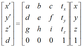
Figure 25. The 4 x 4 matrix for transformation plus translation in 3D.

• The top left block is T, and the last column is t : the 3 x 3 matrix [[a, b, t_x], [c, d, t_y], [0, 0, 1]] carries both parts of p' = Tp + t.
• A pure translation uses T = I : for example, [[1, 0, 2], [0, 1, 0], [0, 0, 1]] moves every point 2 units along x.
• 3D software uses the 4 x 4 form : OpenGL and most 3D graphics software store a transformation as a 4 x 4 matrix of this kind.
• Two worked examples apply these matrices to a cube : see Translation in 3D and Rotation in 3D.

Why does the order of transformations matter ?

Real applications rarely use a single transformation. A robot arm or a 3D scene chains rotations, scalings and translations one after another. With homogeneous coordinates each step is one matrix, and the whole chain is one matrix product. But the order of the factors changes the result, so let's check it on one point.

Let's rotate the point (1, 0) by 90 degrees and translate it by t = [2, 0]^T. In homogeneous form the rotation is R = [[0, -1, 0], [1, 0, 0], [0, 0, 1]], and the translation is M = [[1, 0, 2], [0, 1, 0], [0, 0, 1]]. The rightmost matrix acts first. So M R rotates first and translates second, while R M translates first and rotates second. The block below works out both orders.

Start:                     p = (1, 0)
Rotate, then translate:    R p = (0, 1)      then + t   gives (2, 1)
Translate, then rotate:    p + t = (3, 0)    then R     gives (0, 3)

M R = [ 0  -1   2 ]        R M = [ 0  -1   0 ]
      [ 1   0   0 ]              [ 1   0   2 ]
      [ 0   0   1 ]              [ 0   0   1 ]

The two products differ only in the last column. In M R, the translation stays [2, 0]. In R M, the translation has itself been rotated to [0, 2]. This is the general rule. Translating first and rotating second is the same as rotating first and then translating by the rotated vector.

An affine map with an invertible T can also be undone. Solving p' = Tp + t for p gives p = T^-1(p' - t). For M R above, the inverse is [[0, 1, 0], [-1, 0, 2], [0, 0, 1]]. Applied to (2, 1), it gives back (1, 0). It first moves the point back by t and then rotates it by -90 degrees.

• The rightmost matrix acts first : in M R p, the point meets R before M.
• Rotation and translation do not commute : M R and R M have different translation columns, so they move the same point to different places.
• Two translations always commute : their product simply adds the two translation vectors, in either order.
• A chain collapses into one matrix : multiply the chain once, and then apply the single 3 x 3 or 4 x 4 matrix to every point. This saves work when an object has thousands of vertices.
• The inverse reverses the order : (M R)^-1 = R^-1M^-1. So the translation is undone first and the rotation last.

What does an affine map keep and what does it change ?

Scaling, shear and rotation look very different in the pictures above. Even so, all affine maps share a few properties. These properties tell you which measurements survive a transformation and which ones you must compute again.

An affine map sends straight lines to straight lines, and parallel lines to parallel lines. It also keeps ratios along a line, so the midpoint of a segment maps to the midpoint of the new segment. That is why the grid in Figure 6 is still made of straight, evenly spaced lines after the shear. Lengths and angles behave differently. Only rotations and reflections keep them, because only their matrices are orthogonal, with T^TT = I. Scaling and shear change lengths, and shear also changes angles.

The determinant of T tells you what happens to area in 2D and to volume in 3D. Its size is the area factor, and its sign tells you whether the map makes a mirror image. The table below lists the 2D matrices from this page. The last row adds a projection to show what a zero determinant means.

• Lines stay lines, and parallel lines stay parallel : this holds for every affine map, with or without translation.
• A nonzero translation breaks linearity : T(p₁ + p₂) + t is not equal to (Tp₁ + t) + (Tp₂ + t). The two sides differ by one extra t. That is why the map is called affine rather than linear.
• A negative determinant means a mirror image : Figure 3 and Figure 4 show this case. Reflecting in both axes, as in Figure 5, gives a determinant of +1, which is a rotation by 180 degrees.
• A zero determinant cannot be undone : the map collapses the plane onto a line or a point, so T^-1 does not exist.