As far as I experienced in real field in which we use various kind of engineering softwares in stead of pen and pencil in order to handle various real life problem modeled by differential equations. This would be very important topics but I have seen almost no textbook which touches this kind of topics in detail. In many case, they just shows the final result (a bunch of first order differential equation converted from high order differential equation) but not much about the process.
- What does the conversion produce, and why is it needed ?
- Example : 3rd Order Homogeneous Lineare Differential Equation - System with no external input
- Example : 3rd Order Non-Homogeneous Lineare Differential Equation - System with Single External Input
- Example : Simultaneous Differential Equation - System Equation
- How is a converted system checked ?
- Example from YouTube
What does the conversion produce, and why is it needed ?
Let's assume that we have a higher order differential equation (3rd order in this case). The goal is to replace this one equation of order three with three equations of order one. Each new equation holds only a first derivative, and the three together carry the same information as the original equation.

Our goal is to convert these higher order equation into a matrix equation as shown below which is made up of a set of first order differential equations.

We will look into the process of the conversion through some examples in this section, but before going there, I want to mention a little bit about why we need this kind of conversion.
Why do we want this kind of conversion ? Just to give us another type of headache ? Of course not -:)
As shown in the following illustration, once we get a bunch of first order differential equations out of Higher order equation, we can
i) use them more easily for numerical processing to solve the problem (See Differential Equation pages of Matlab/Octave)
ii) convert into a matrix form in which we can use a lot of linear algebra tools to analyze/solve the equation
iii) (Mostly in Control System theory) convert into a state space model which can be analyzed by various tools specially designed for State Space analysis tool. (See Differential Equation pages of Matlab/Octave)

The diagram shows the three uses side by side. The first order system in the middle row feeds a numerical solver, a matrix equation and a state space model. All three start from the same set of first order equations, so the conversion is done once and then serves all of them.
An n-th order equation becomes n first order equations : The new variables are y and its derivatives up to order n - 1, so the count of unknowns equals the order.Numerical solvers expect first order systems : Most ODE solvers take dx/dt = f(t, x), so a higher order equation has to be converted before it can be solved numerically.The matrix form opens linear algebra : Once the system is written as dx/dt = Ax, the eigenvalues of A describe the behavior of the solution.
Now let's look into the detailed process for this conversion through following examples.
Example : 3rd Order Homogeneous Lineare Differential Equation - System with no external input
This first example has no input term on the right side, so the system moves only because of its initial conditions. It is the simplest case, and the next two examples add an input and a second unknown function. Let's assume that we have a 3rd order differential equation as follows.

There can be several different way for the conversion, but my trick is like this. First, I look for the order of the equation and replace all the terms of lower than the order with different variables. Since this is 3rd order differential equation, I will replace 2nd, 1st, 0th term with other variables as shown below.


You can also do this replacement process as shown below. The method shown above would give you mathematical meaning of the replacement process, but once you fully understand the mathematical meaning the method shown below would be a handy shortcut for this process.

As you see above, I replaced the 0th, 1st, 2nd order term with x1,x2,x3 respectively. If we plug in these variable into the original equation and do a little bit of rearrangement, we get the following equation.

If you collect all the equations which is the first order, you would get following three equations. In this case, the first two equations were directly from our definition and the third one is from original equation.

This is the end of the process, if you want to solve this differential equations in a numerical method as explained in this page. But if you want to convert this set of simultaneous equations into a matrix form, it would be good to revise the equations as follows.

Now you will easily convert these simulteneous equation into a matrix form as follows.

The matrix A has a fixed pattern. Ones sit just above the diagonal, and the coefficients of the original equation, with a minus sign, fill the last row. This pattern is called the companion matrix of the equation. The first two rows only repeat the definitions of the new variables, and the last row carries the physics of the original equation.
The first rows are definitions : dx1/dt = x2 and dx2/dt = x3 come from the substitution, not from the equation.The last row is the original equation : It holds -a0, -a1 and -a2, in the order of x1, x2 and x3.The zeros are part of the structure : Writing 0x1 and 0x3 explicitly is what lets each equation become one row of the matrix.
Example : 3rd Order Non-Homogeneous Lineare Differential Equation - System with Single External Input
Now I have another equation. This is almost same as the first equation but only one minor diference. (I would strongly recommend you to go through the first example before you go through this example).

As we did in the first example. I look for the order of the equation and replace all the terms of lower than the order with different variables. Since this is 3rd order differential equation, I will replace 2nd, 1st, 0th term with other variables as shown below.


Here goes the second method again. You can pick whatever method you like.

As you see above, I replaced the 0th, 1st, 2nd order term with x1,x2,x3 respectively. If we plug in these variable into the original equation and do a little bit of rearrangement, we get the following equation.

If you collect all the equations which is the first order, you would get following three equations. In this case, the first two equations were directly from our definition and the third one is from original equation.

This is the end of the process, if you want to solve this differential equations in a numerical method as explained in this page. But if you want to convert this set of simultaneous equations into a matrix form, it would be good to revise the equations as follows.

Now you will easily convert these simulteneous equation into a matrix form as follows.

From the equation above, you lost y(t). You can express y(t) in generic form as follows.

Now you have to figure out unknown values marked above. You can figure out those unknown values as shown below.
![Output y = x1 gives C = [1 0 0] and no u(t) term](../image/EngMath_DifferentialEq_HigherOderToFirstOder_Ex_2ndOrderLinearHomogenous_2_09.png)
Combining the two matrix equations that we built from the long procedure described above, you can have a set of matrix as shown below. This form of matrix equation is called 'State Space' matrix equation.
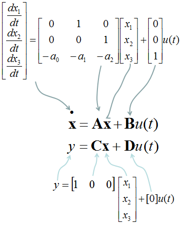
The input u(t) changes only the last equation, because the original equation holds u(t) on its right side. So B = [0 0 1]T, and A is the same companion matrix as in the homogeneous example. The output y is the original unknown y(t) = x1, so C = [1 0 0] and D = [0].
One label in the diagram that introduces y = Cx + Du(t) needs care. The unknown entry of D is written there as [c1], the same name as the first entry of C. It is a separate value, the direct gain from u(t) to y. It turns out to be 0 in this example, as the state space summary at the end of this section shows. Also, the note under x calls it a known vector. x is the state vector, and it is known in the sense that the state equation computes it.
The input enters through B : B has a 1 in the row whose equation contains u(t) and zeros elsewhere.The output is chosen through C : C picks the state variable that you want to observe. Here it picks x1 = y(t).D is zero for this equation : The output y(t) does not depend on u(t) directly. u(t) affects y(t) only through the state.
Example : Simultaneous Differential Equation - System Equation
Previous example shows how we can convert one higher linear order differential equation into a single matrix equation. In this example, I will show you the process of converting two higher order linear differential equation into a sinble matrix equation. If you extend this procedure, you can convert any number of higher order differential equations into a single matrix equation.

You see two variables (more specification, two functions x(t) and y(t)) in this equations and two differential terms x''(t), y''(t). Now let'sdefine these functions and differentials as follows.

If you substitue the original equations with the variables that you defined above, you get a new equations as follows.

If you combine the new equations and your definitions so that first order diffential forms are at the left side and all the remaining terms are on the right side.

Now you can convert the above equations into the following format. Do you know why I am doing this kind of conversion using many of '0' terms which does not have much meaning in mathematical sense ?
It is to convert this simultaneous equations into the matrix form.

Now you can easily convert this equation into a matrix form as shown below.

Two second order equations give four first order equations, one for each of x, x', y and y'. The constant terms 1 and 5 do not multiply any state variable, so they form a separate constant vector next to the matrix. They act in the same way as the input u(t) of the previous example, with a constant input.
The number of state variables is the sum of the orders : Two equations of order 2 give 2 + 2 = 4 state variables.Coupling appears off the diagonal blocks : The entries 5 and 25 connect the x equations with the y equations. Without them, the matrix would split into two independent 2 x 2 blocks.Constant terms form a separate vector : The vector [0 1 0 5]T is added to Ax, and it does not change the eigenvalues of the system.
How is a converted system checked ?
A conversion with many substitutions is easy to get wrong by one sign or one index. Let's use two checks that need no solving: the eigenvalues must match the original equation, and the equilibrium must match it too.
For the 3rd order example, the characteristic polynomial of the companion matrix is det(sI - A) = s3 + a2s2 + a1s + a0. This is exactly the characteristic equation that you get by putting y = est into the original equation. For example, with a2 = 6, a1 = 11 and a0 = 6, the eigenvalues of A are -1, -2 and -3. These are the roots of s3 + 6s2 + 11s + 6 = (s + 1)(s + 2)(s + 3).
For the simultaneous example, the equilibrium is where every derivative is zero. The original equations then give 7x - 5y = 1 and -25x + 5y = 5, so x = -1/3 and y = -2/3. The matrix form gives the same point, x1 = -1/3 and x3 = -2/3, with x2 = x4 = 0. The characteristic polynomial of the 4 x 4 matrix is s4 + 12s2 - 90. Its roots are about +/-2.286 and +/-4.150j. The positive real root means that this system moves away from its equilibrium, so a small disturbance grows instead of dying out.
The eigenvalues of A are the roots of the characteristic equation : A correct conversion keeps them unchanged, so comparing the two is a quick test.The equilibrium must agree : Setting all derivatives to zero in the original equations and in the matrix form must give the same point.The trace is another quick test : The sum of the eigenvalues equals the trace of A. For the companion matrix it is -a2, and for the 4 x 4 example it is 0.
Example from YouTube
The linked lecture takes the next step after the conversion on this page. It solves the first order system du/dt = Au with the matrix exponential eAt, and it uses the eigenvalues of A in the same way as the check in the previous section.