This page collects Matlab/Octave examples that solve differential equations numerically. Each example follows the same path. It starts from the model equation, rewrites it into the form the solver expects, runs the code and shows the output plot.

Three tools appear on the page. The first, ode45, integrates a system of first order equations dy/dt = f(t,y) from an initial condition. The second, lsim, simulates a linear state space model driven by an input signal. The third, step, plots the step response of a transfer function. Where a picture or a listing contains a mistake, the text next to it points out the mistake, and the listing itself is left as it was run.

• ODE45
  • ode45 - 1st order
  • ode45 - Undamped Pendulum
  • ode45 - Single Spring Mass- Undamped
  • ode45 - Single Spring Mass- Damped
  • ode45 - Single Spring Mass- Damped and External Force
  • ode45 - Single Spring Mass- Damped and External Force with Frequency Sweep
  • ode45 - 1st Order System Equation- Lorenz Attractor
  • ode45 - Chemical Reaction
  • Ode45 - Van der Pol Oscillator
  • Ode45 - Van der Pol Oscillator with External Force
  • Ode45 - Duffing Oscillator
  • Ode45 - Matrix Equation - 2 x 2
• Lsim-State Space Model
  • Lsim - Damped Spring
  • Lsim - RLC Circuit
• Step
  • Step - 1/s
  • Step - 1 over a*s+1
  • Step - 1 over a*s²+b*s+1

ODE45

Most differential equations in engineering have no closed form solution, or have one that is hard to find. The ode45 function solves them numerically, so you only need to describe the equation and give a starting point. Let's first look at what ode45 expects, because every example below uses the same four inputs.

ode45 solves an initial value problem of the form dy/dt = f(t,y) with y(t₀) = y₀. Here y can be a scalar or a column vector. The solver is an explicit Runge-Kutta method with a 4th and 5th order pair, known as the Dormand-Prince pair. It compares the two estimates at each step to control the error, and it changes the step size automatically.

A call has the form [t,y] = ode45(f, tspan, y0, options). The first input is the function that returns dy/dt. The second is the time range, for example [0 25]. The third is the initial condition, with one value per state variable. The fourth is an optional structure made by odeset. The output t is a column vector of time points. The output y has one row per time point and one column per state variable, so y(:,1) is the first state and y(:,2) is the second.

ode45 accepts only first order equations, so a second order equation has to be rewritten first. The standard method is to name the unknown y₁ and its derivative y₂. Then dy₁/dt = y₂, and the original equation gives dy₂/dt. Most examples below draw this step as a picture before the code.

Every example uses the same options: odeset('RelTol', 0.00001, 'AbsTol', 0.00001, 'InitialStep', 0.5, 'MaxStep', 0.5). RelTol and AbsTol set the error tolerances. They are much tighter than the defaults of 10^-3 and 10^-6. MaxStep stops the solver from taking a step longer than 0.5, so the plotted curves stay smooth even where the solution changes slowly.

• ode45 needs four things : a derivative function, a time span, an initial condition and, optionally, an odeset structure.
• Higher order equations must be reduced first : an n-th order equation becomes n first order equations, one per state variable.
• Column k of y is state k : plot y(:,1) against y(:,2) to get the phase plot that most examples below show.

ode45 - 1st order

The simplest case is a single first order equation, dy/dt = -2y with y(0) = 2. Its exact solution is y(t) = 2e^-2t, so you can check the numerical result against a known answer. The annotated picture below maps each part of the equation onto the Matlab call.

Ex)

The plot starts at y = 2 at t = 0, which is the initial condition, and decays toward zero. At t = 1 the exact value is 2e^-2 = 0.271. The curve falls below 1% of its start value after t = ln(100)/2 = 2.3. This is why the curve looks flat from about t = 3 onward, even though the time span runs to 5.

• The listing uses inline : inline() is a legacy function in both Matlab and Octave. The anonymous function f = @(t,y) -2*y does the same job, and every later example uses that form.
• The decay rate is the coefficient : for dy/dt = -ay the solution falls by a factor of e every 1/a time units, here every 0.5.

ode45 - Undamped Pendulum

An undamped pendulum obeys d²θ/dt² = -ω² sin(θ). This equation is second order and nonlinear, so it is a good first test of the order reduction step. The picture below sets θ = y₁ and dθ/dt = y₂. It then copies the two right hand sides into dy_dt.

In the call annotation above, the two initial condition labels carry the wrong values. The vector [0.0 1.0] means y₁(0) = 0.0 and y₂(0) = 1.0. So the pendulum starts at the bottom, θ = 0, with an angular velocity of 1.

Ex 1)

Energy conservation gives the peak angle of Ex 1. With y₂(0) = 1 and ω = 1, 1 - cos(θ_max) = y₂(0)²/2 = 0.5, so θ_max = 60 deg = 1.047 rad. The red curve peaks at about 1.05, which matches. The period is 6.74, about 7% longer than the small angle value 2π = 6.28, because sin(θ) grows more slowly than θ.

The listing labels the phase plot axes with xlabel('y(2)') and ylabel('y(1)'). But plot(y(:,1),y(:,2)) puts y₁ on the horizontal axis. So read the horizontal axis as the angle y₁ and the vertical axis as the angular velocity y₂. The spring examples that follow have the same swap.

Ex 2) If you change the initial condition, you would get different result (a little bit distorted circle)

With y₂(0) = 1.7, the same energy calculation gives 1 - cos(θ_max) = 1.445, so θ_max = 2.03 rad, or 116 deg. The pendulum now swings well above horizontal. The period grows to 8.44, and the phase plot is no longer a circle. This is the distortion that the Ex 2 note describes. If y₂(0) reaches 2, the pendulum just reaches the top. Above 2, it rotates over the top instead of swinging.

• Energy fixes the amplitude : for the undamped pendulum, y₂²/2 + ω²(1 - cos y₁) stays constant. So the peak angle follows from the initial velocity alone.
• The period depends on amplitude : it is 6.74 at 60 deg and 8.44 at 116 deg, against 6.28 for the linearised pendulum.
• y₂(0) = 2 is the separatrix : with ω = 1, this initial velocity carries the pendulum exactly to the top.

ode45 - Single Spring Mass- Undamped

A mass on a spring without damping obeys m d²x/dt² + kx = 0. This is the linear version of the pendulum, so let's compare the two plots. The picture below reduces the equation to two first order equations in the same way, with y₁ = x and y₂ = dx/dt.

In the call annotation above, the label texts are correct: y₁(0) = 0.0 and y₂(0) = 1.0. But the two arrows point at each other's value. The first element of the vector is always y₁(0).

Ex)

With m = k = 1, the natural frequency is ω_n = √(k/m) = 1 rad/s and the period is 2π = 6.28. The exact solution for y₁(0) = 0 and y₂(0) = 1 is x(t) = sin(t), and the velocity is cos(t). This is why the phase plot is a circle of radius 1. Compare it with the pendulum Ex 1, which starts from the same state. The pendulum reaches 1.05 instead of 1.0, and it takes 6.74 instead of 6.28 per cycle.

• The linear oscillator conserves energy : kx²/2 + mv²/2 is constant, so the phase plot is a closed ellipse, and a circle when k = m.
• The period does not depend on amplitude : it is 2π√(m/k) for any initial condition. The pendulum loses this property at large angles.

ode45 - Single Spring Mass- Damped

Adding a damper adds a term proportional to velocity: m d²x/dt² + c dx/dt + kx = 0. The only change in the code is the extra term -(c/m) * y(2) in the second row. The picture below shows where that term lands after the order reduction.

The call annotation above is the same image as in the undamped example, with the same swapped arrows. The initial state is again y₁(0) = 0 and y₂(0) = 1.

Ex)

The damping ratio is ζ = c/(2√(km)) = 0.15. This is well below 1, so the system is underdamped and still oscillates. The amplitude envelope decays as e^-0.15t, and by t = 25 it has fallen to 0.024 of its initial value. The damped frequency is ω_n√(1 - ζ²) = 0.989 rad/s, so the period grows only slightly, to 6.36. In the phase plot, the circle of the undamped case becomes a spiral that winds into the origin.

• ζ decides the shape : ζ below 1 oscillates, ζ = 1 is critically damped, and ζ above 1 returns to rest without overshoot.
• Light damping barely changes the frequency : at ζ = 0.15 the period changes by about 1%, while the amplitude falls by a factor of about 40 over the plotted 25 time units.

ode45 - Single Spring Mass- Damped and External Force

Now let's drive the damped spring with a periodic external force. The model becomes m d²x/dt² + c dx/dt + kx = F₀ cos(ωt). The forcing term appears as (F0/m) * cos(w*t) in the second row of dy_dt. The anonymous function now uses t directly, so the right hand side changes with time.

The top line of the picture above writes the force as F₀ sin(ωt), while the state equations and the code use cos(ωt). The code produced the plot, so read the force as F₀ cos(ωt). The choice only shifts the phase of the steady state response, not its amplitude.

Ex)

The response has two parts. The transient comes from the initial condition and dies out as e^-0.15t, the same envelope as in the unforced example. The steady state oscillates at the driving frequency ω = 2.5, not at the natural frequency 1. Its amplitude is X = F₀/√((k - mω²)² + (cω)²) = 0.5/5.30 = 0.094, and the velocity amplitude is Xω = 0.236. These values match the plot after about t = 20. In the phase plot, the steady state is the small closed loop in the middle.

• The steady state follows the driver : after the transient, the mass moves at the forcing frequency, whatever its natural frequency is.
• Driving above resonance gives a small response : at ω = 2.5 the inertia term mω² = 6.25 dominates the stiffness k = 1. So the amplitude is less than a fifth of the static deflection F₀/k = 0.5, and the motion lags the force by 172 deg.

ode45 - Single Spring Mass- Damped and External Force with Frequency Sweep

A single forcing frequency shows one point of the frequency response. This example repeats the forced simulation for ten frequencies, ω = 0.2, 0.4, ... 2.0, so you can see where the spring resonates. The spring is softer here, k = 0.7, and the mass starts at rest.

Ex)

Each row of the output is one frequency, from 0.2 at the top to 2.0 at the bottom. The wide panel shows y₁ and y₂ against time up to t = 100, and the small panel on the right is the phase plot. The listing hides the tick labels, so the table below gives the steady state amplitude of each row. It is computed from X = F₀/√((k - mω²)² + (cω)²) with m = 1, k = 0.7, c = 0.3 and F₀ = 0.5.

The natural frequency is √(k/m) = 0.837 rad/s. The amplitude peak sits slightly lower, at √(k/m - c²/(2m²)) = 0.809 rad/s. Row 4, ω = 0.8, is closest to that peak. Its amplitude of 2.02 slightly exceeds the ylim of [-2 2] in the listing. Above resonance the amplitude falls quickly, to 0.149 at ω = 2.0. With c = 0.3 the start-up transient decays as e^-0.15t, so it takes about 30 time units to fall below 1%.

• Resonance is where the curve peaks : the response at ω = 0.8 is 2.7 times the response at ω = 0.2 and 14 times the response at ω = 2.0.
• A sweep needs a settle time : read each amplitude after the transient has decayed, here after about t = 30.

ode45 - 1st Order System Equation- Lorenz Attractor

The Lorenz system is three coupled first order equations, so no order reduction is needed. It is a classic example of a deterministic system with chaotic behaviour. The picture below maps x, y and z onto y₁, y₂ and y₃, and each right hand side onto one row of dy_dt.

Ex)

The parameters P = 10, r = 28 and b = 8/3 are the standard values that Lorenz used. P is often written σ. For these values the system has three equilibrium points. They are the origin, (8.49, 8.49, 27) and (-8.49, -8.49, 27), from x = y = +/-√(b(r - 1)) and z = r - 1. All three equilibria are unstable, so the trajectory never settles. Instead it circles one of the two outer equilibria for a few turns and then switches to the other one, at irregular times.

The three panels project the attractor onto the y₁-y₂, y₂-y₃ and y₁-y₃ planes. The two holes in each panel sit at the two outer equilibria.

• Chaos means sensitive dependence : two starting points that differ by a tiny amount separate quickly. So the detailed curve depends on the solver tolerances, but the shape of the attractor does not.
• Tight tolerances help only for a while : a RelTol of 10^-5 keeps the orbit accurate for some time, but no tolerance makes a 250 time unit trajectory exact in detail.

ode45 - Chemical Reaction

A chemical reaction network is a natural system of first order equations. Here A turns into B at rate k₁, B turns back into A at rate k₂, and B turns into the final product C at rate k₃. Each concentration becomes one state variable, as the picture below shows.

Ex)

The simulation starts with pure A, so y = [1 0 0]. A falls fast at first, and B builds up to a peak of 0.535 at t = 0.36. C grows steadily as B converts into it, and by t = 4 it has reached 0.928. The sum A + B + C stays at 1 for all t, because the three right hand sides add up to zero. That makes a useful check on any numerical solution of a closed reaction.

The A and B equations do not depend on C, so they form a 2 x 2 linear system with the matrix [-5 2; 5 -3]. Its eigenvalues are -0.68 and -7.32. The fast eigenvalue explains the quick early drop of A. The slow one sets how long C takes to approach 1.

In the Octave legend, the colour samples for y(2) and y(3) do not match the curves. The code plots y(2) in green and y(3) in blue. So the green curve that peaks is B, and the blue curve that rises toward 1 is C.

• Mass is conserved : dA/dt + dB/dt + dC/dt = 0, so y(1) + y(2) + y(3) = 1 at every step.
• The reaction has two time scales : the eigenvalues -7.32 and -0.68 give a fast phase of about 0.14 time units and a slow phase of about 1.5.

Ode45 - Van der Pol Oscillator

The Van der Pol oscillator has a damping term that changes sign with amplitude: d²x/dt² - μ(1 - x²) dx/dt + kx = 0. When |x| is below 1, the term pumps energy in. When |x| is above 1, it takes energy out. The order reduction in the picture below follows the same pattern as the spring examples.

The call annotation above has the same arrow swap as the spring examples. The label text is correct: y₁(0) = 1.0 and y₂(0) = 2.0.

Ex)

Whatever the start state, the solution settles onto one closed curve, called a limit cycle. For μ = 1 and k = 1, the limit cycle has an amplitude of about 2.01 in y₁ and 2.68 in y₂, and a period of 6.66. The plot reaches this cycle within the first turn. This is why the phase plot shows a single loop with a short tail. Compare this with the linear damped spring, whose spiral always ends at the origin.

• A limit cycle is an isolated closed orbit : trajectories inside it grow and trajectories outside it shrink, until both reach it.
• The equation sets the amplitude : the limit cycle amplitude is about 2 whatever the initial condition. A linear oscillator instead keeps the amplitude of its start state.

Ode45 - Van der Pol Oscillator with External Force

This example adds a periodic force A sin(ωt) to the Van der Pol oscillator, with A = 2 and ω = 10. The forcing frequency is about ten times the limit cycle frequency. So let's see how much a fast force disturbs the slow oscillation.

The call annotation above is reused from the unforced example. The start state is the same, y₁(0) = 1.0 and y₂(0) = 2.0.

Ex)

The slow limit cycle survives almost unchanged. The state y₁ still swings between about -2 and 2 with a period near 6.7. The fast force shows up as a ripple. For a force much faster than the system, the velocity ripple is about A/ω = 0.2 and the position ripple is about A/ω² = 0.02. That is why the green y₂ curve looks noisy while the red y₁ curve stays smooth. It is also why the phase plot becomes a band of slightly shifted loops.

• Inertia filters a fast force : the position responds to a force at frequency ω with an amplitude of roughly A/ω².
• A slow force acts differently : when ω is close to the limit cycle frequency, the oscillator can lock to the driver frequency. This is called entrainment.

Ode45 - Duffing Oscillator

The Duffing oscillator adds a cubic spring term to the forced, damped spring: d²x/dt² + δ dx/dt + βx³ + ω₀²x = γ cos(ωt + φ). With β greater than 0, the cubic term makes the spring stiffer as the displacement grows. The picture below reduces the equation to two first order equations.

In the last line of the picture above, the spring terms are written with y. They mean y₁, as in the code.

The vector [3.0 4.1] means y₁(0) = 3.0 and y₂(0) = 4.1. The values in brackets in the annotation above are right, but the words for y1 and for y2 are swapped.

Ex)

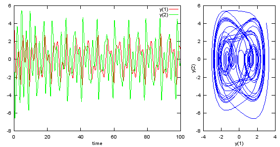
With a strong force, γ = 6, and light damping, δ = 0.06, the response does not settle into a simple repeating cycle within 100 time units. The phase plot shows the trajectory crossing itself many times, with loops of many different sizes. Lightly damped, strongly driven Duffing oscillators are a standard example of chaotic motion. But a 100 time unit plot alone cannot prove chaos for these parameters. A longer run, or two runs from nearby initial conditions, would show whether the motion is chaotic or a long transient.

• The cubic spring makes the frequency depend on amplitude : with β greater than 0 the spring hardens, so larger swings oscillate faster.
• Irregular output needs a check : repeat the run with a slightly different initial condition. If the two curves separate quickly, the motion is sensitive to the start state.

Ode45 - Matrix Equation - 2 x 2

A linear system of first order equations can be written as one matrix equation, dx/dt = Mx. The ode45 function accepts this form directly, because M*y returns the column vector of derivatives. The picture below shows the system and its initial condition x(0) = [1 1]^T.

Ex)

The eigenvalues of M = [-1 -1; 1 -2] are -1.5 +/- j0.866. The negative real part makes both states decay as e^-1.5t. The imaginary part makes them rotate with a period of 2π/0.866 = 7.26. But the decay is so fast that only a small part of one turn is visible. You can see that part in y₁: the red curve drops slightly below zero, to -0.038 at t = 1.81, and then returns toward zero. At t = 4 both states are below 0.003 in magnitude. The legend shows y(1) in black, but the code plots y(1) in red.

• The eigenvalues predict the plot : the real part gives the decay rate, and the imaginary part gives the oscillation frequency.
• A linear system also has an exact solution : x(t) = e^Mtx(0), which expm(M*t)*[1;1] evaluates in Matlab and Octave. The ode45 code is still useful, because it keeps working when M*y is replaced by a nonlinear function.

Lsim-State Space Model

ode45 treats every model as a general nonlinear function. When the model is linear, a state space model describes it more compactly, and lsim simulates it with any input signal you supply. This section runs two linear models that are derived on the State Space Model page.

A state space model has the form dx/dt = Ax + Bu and y = Cx + Du. Here x is the state vector, u is the input and y is the output. The matrix C picks which combination of states you want to see, so the same model can report position, velocity or both. In Octave the model is created with sys = ss(A,B,C,D). Then [y,t,x] = lsim(sys,u,t,x0) returns the output, the time vector and the state history. The input u needs one value per time point.

• C selects the output : C = [1 0] reports the first state and C = [0 1] reports the second, with the same A and B.
• x0 sets the start state : with u = 0, the plot is purely the free response from x0.

Lsim - Damped Spring

The damped spring from the ode45 section returns here as a state space model with m = 1, c = 0.2 and k = 1. The input force is zero, so the plot shows the free response from the start state x0 = [1 0]. This means the mass starts at x = 1 with zero velocity.

Ex) See Damped Spring Example in State Space Model page for the description of the model.

In the picture above, A is the system matrix [0 1; -k/m -c/m], and B = [0; 1/m] is the input matrix. C = [0 1] selects the velocity, and D = 0 because the force has no direct path to the output.

The velocity starts at zero and first goes negative, to -0.86 at t = 1.48, because the stretched spring pulls the mass back toward x = 0. With ζ = c/(2√(km)) = 0.1, the oscillation decays as e^-0.1t and has a period of 6.31.

Ex)

This second example changes only C, to [1 0], so the output is now the position x.

The position starts at 1 and swings to -0.73 at t = 3.16, about half a period later. The listing still writes ylabel('velocity'), so the vertical axis label of this plot is wrong. It shows the position. Both plots decay with the same envelope, because they come from the same A matrix.

• Position and velocity are a quarter period apart : for light damping, the velocity peaks close to where the position crosses zero.
• The plot label does not follow C : ylabel is fixed text, so change it whenever you change C.

Lsim - RLC Circuit

A series RLC circuit is the electrical twin of the damped spring. The two states are the capacitor voltage v2 and its derivative. The input u is the source voltage, and the listing switches it off for two time units to create two voltage steps.

Ex)  See RLC Circuit Example in State Space Model page for the description of the model.

In the picture above, the second row of A holds -1/(LC) and -R/L, and B = [0; 1/(LC)]. The output matrix [1 0] selects x₁, the capacitor voltage v2.

With R = 1, L = 0.1 and C = 0.01, the natural frequency is 1/√(LC) = 31.6 rad/s, and the damping ratio is (R/2)√(C/L) = 0.158. So each step makes the voltage ring with a period of about 0.2 time units and an overshoot of 60%. The plot shows this. The output falls to about -0.6 after the step down near t = 2, and it rises to about 1.6 after the step up near t = 4. The step times are 1.99 and 3.99, because u(200:400) = 0 clears samples 200 to 400 of t = 0:0.01:10. Before the first step there is no transient, because x0 = [1 0] already equals the steady state for u = 1.

The listing uses the name C twice. It is first the capacitance and then the output matrix. The code works because A and B are computed before C is overwritten, but the reuse breaks easily when the lines are reordered.

• It is the same equation with different names : L, R and 1/C play the roles of m, c and k in the spring.
• A low ζ means strong ringing : ζ = 0.158 gives a 60% overshoot on each step.

Step

Sometimes you only need to know how a linear system reacts when its input jumps from 0 to 1. The step function answers this directly from a transfer function. You do not need state equations or an ODE solver for it.

A transfer function is the ratio of output to input in the Laplace domain. The function tf(num, den) builds one from the coefficient vectors of the numerator and the denominator, in descending powers of s. For example, tf([1],[1 0]) is 1/s. step(sys) plots the output for a unit step input with zero initial conditions, and step(sys, Tfinal) sets the end time. The three examples below go from the simplest system, a pure integrator, to a second order system with overshoot.

• The final value comes from s = 0 : when the system is stable, the step response settles at the value of the transfer function at s = 0. This value is 1 for the two lower examples.
• The poles give the shape : a single real pole gives an exponential rise, and a complex pair gives an oscillating rise.

Step - 1/s

1/s is a pure integrator. Its output is the running integral of the input, so a unit step input produces a ramp. The Octave output below first prints the transfer function and then plots the response.

Ex)

The plot is a straight line with slope 1, and it reaches 10 at t = 10. The response never settles, because the integrator has a pole at s = 0. So the final value rule of the Step section does not apply to it.

Step - 1 over a*s+1

The first order lag 1/(τs + 1) describes a system with one energy store, such as an RC circuit. The listing uses τ = 0.5, so the pole is at s = -2 and the response should settle within a few multiples of 0.5.

Ex)

The step response is y(t) = 1 - e^-t/τ. It reaches 63.2% of the final value at t = τ = 0.5 and 98.2% at t = 4τ = 2. The plot matches this. It is near 0.63 at t = 0.5 and nearly flat at 1 after t = 2.

Step - 1 over a*s²+b*s+1

A second order denominator gives a pair of poles. With a = 1.5 and b = 0.7, the poles are complex, so the step response overshoots and rings before it settles.

Ex)

Compare the denominator with the standard form s²/ω_n² + 2ζs/ω_n + 1. This gives ω_n = 1/√a = 0.816 rad/s and ζ = b/(2√a) = 0.286. The peak overshoot is e^{-πζ/√(1 - ζ2)} = 39%, at t = π/(ω_n√(1 - ζ²)) = 4.0. The plot peaks at about 1.39 near t = 4, which matches. The 2% settling time is 4/(ζω_n) = 17. This explains why the curve is still slightly off 1 near t = 16.