Python - Image Handling
Python offers multiple libraries for image handling and manipulation, allowing you to perform a variety of operations on images, such as reading, writing, resizing, filtering, and transforming. These libraries provide a powerful set of tools for working with image data, making it easy to create, process, and analyze images in your Python applications.
Some popular Python libraries for image handling and manipulation are:
- Pillow (PIL - Python Imaging Library): Pillow is a widely-used, user-friendly library that supports a range of image file formats. It provides functions for opening, saving, and manipulating images, as well as for applying various filters and transformations. Pillow is an easy-to-use library suitable for beginners and experts alike.
- OpenCV: OpenCV (Open Source Computer Vision) is a powerful library primarily designed for computer vision tasks but also supports various image processing operations. OpenCV offers advanced features such as object recognition, feature detection, and tracking. It is ideal for building sophisticated applications that require real-time image processing or computer vision capabilities.
- scikit-image: scikit-image is a library built on top of NumPy, SciPy, and matplotlib, focusing on image processing. It offers a collection of algorithms for image processing, such as edge detection, segmentation, and morphological operations. scikit-image is suitable for users who need advanced image processing functionality and are familiar with the scientific Python ecosystem.
- ImageMagick: ImageMagick is a versatile command-line tool for image manipulation that also provides Python bindings through the Wand library. ImageMagick supports various image formats and offers powerful features like image conversion, resizing, and filtering. The Wand library makes it easy to access ImageMagick's functionality from Python code.
- Matplotlib : Matplotlib is a popular Python library for data visualization and plotting, which can also be used for basic image processing tasks. Matplotlib offers functions for reading, displaying, and saving images, as well as basic manipulation like resizing, cropping, and color mapping. While Matplotlib is not specifically designed for image processing like some other libraries (e.g., Pillow or OpenCV), it is useful for working with images in the context of data visualization and analysis. For example, you can use Matplotlib to display images alongside plots, create image-based visualizations, or preprocess images for use in other data analysis tasks. However, for more advanced image processing tasks or computer vision applications, specialized libraries like OpenCV or scikit-image are more suitable.
Followings are list of topics and examples on this note.
- PIL/matplotlig
- Reading and Displaying Image with PIL
- Reading and Displaying Image with matplotlib
- Resizing the Image
- Rotating the Image
- Cropping the Image
- Converting the Image Color
- Image to Array and Array to Image
- Cropping image from Array
- Splitting an Image into Color Layers
- Saving the Image
- OpenCV
Reading and Displaying Image with PIL
|
# Import the required libraries # Import the Python Imaging Library (PIL) import PIL # Import the Image module from PIL from PIL import Image
#Open the image file #Open the image with the specified filename img = Image.open('Scene_01.png')
#Print image details #Print the image format, mode, and size print('Format = ', img.format, ' ,Mode = ', img.mode, ' ,Size = ', img.size)
#Display the image img.show() # Show the image in the default image viewer |
|
|
Reading and Displaying Image with matplotlib
|
from matplotlib import image from matplotlib import pyplot
img = image.imread('Scene_01.png')
print('Data Type = ',img.dtype,' ,Size = ', img.shape)
pyplot.imshow(img) pyplot.show() |
|
Data Type = float32 ,Size = (734, 1137, 4)
|

|
import PIL from PIL import Image
img = Image.open('Scene_01.png')
print('Format = ',img.format, ' ,Mode = ',img.mode, ' ,Size = ', img.size)
img.show() |
|
Format = PNG ,Mode = RGBA ,Size = (1137, 734)
|
|
img_resized = img.resize((200,200)); print('Format = ',img_resized.format, ' ,Mode = ',img_resized.mode, ' ,Size = ', img_resized.size)
img_resized.show() |
|
Format = None ,Mode = RGBA ,Size = (200, 200)
|

|
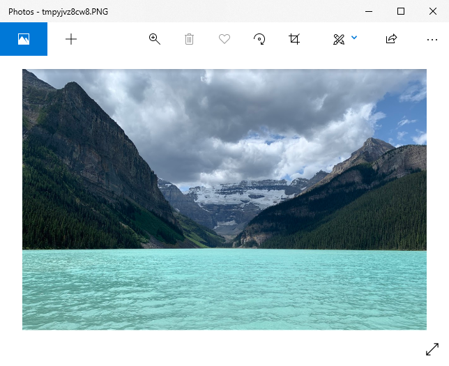
import PIL from PIL import Image from matplotlib import pyplot
img = Image.open('Scene_01.png')
pyplot.subplot(1,3,1) pyplot.imshow(img)
pyplot.subplot(1,3,2) rot45 = img.rotate(45); pyplot.imshow(rot45)
pyplot.subplot(1,3,3) rot90 = img.rotate(90); pyplot.imshow(rot90)
pyplot.show() |
|
|

|
import PIL from PIL import Image from matplotlib import pyplot
img = Image.open('Scene_01.png')
pyplot.subplot(1,3,1) pyplot.imshow(img)
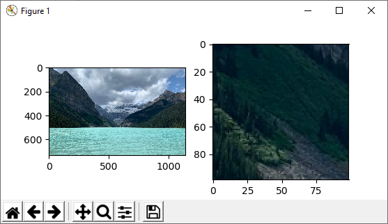
pyplot.subplot(1,3,2) cImg01 = img.crop((200,100,300,200)); pyplot.imshow(cImg01)
pyplot.subplot(1,3,3) cImg02 = img.crop((200,200,600,600)); pyplot.imshow(cImg02)
pyplot.show() |
|
|
|
import PIL from PIL import Image from matplotlib import pyplot
img = Image.open('Scene_01.png')
pyplot.subplot(1,2,1) pyplot.imshow(img)
pyplot.subplot(1,2,2) imgGray = img.convert(mode='L') pyplot.imshow(imgGray)
pyplot.show() |
|
|

Image to Array, Array to Image
|
# Import the required libraries import PIL from PIL import Image from matplotlib import pyplot from numpy import asarray
# Open the image file img = Image.open('Scene_01.png')
# Convert image to numpy array imgAry = asarray(img)
# Print the array size and shape # Print the size and shape of the array print('Size = ', imgAry.size, ',shape=', imgAry.shape)
# Print the first row of the array # Print the first row of the image array print(imgAry[0])
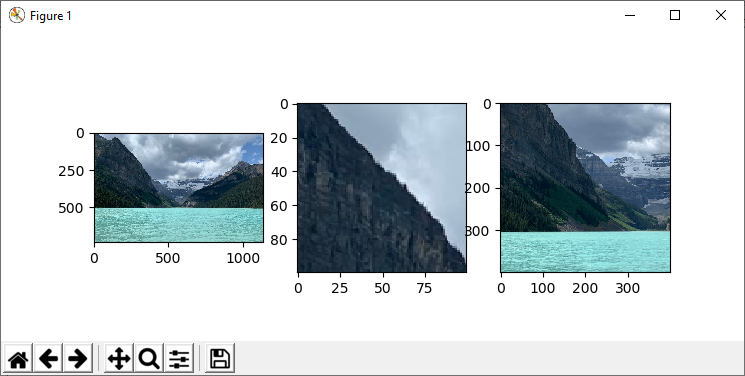
# Modify the array values # Multiply the array by 2 and subtract 100 from each element imgAry = 2 * imgAry - 100
# Convert the modified array back to an image # Create a new image from the modified array mImg = Image.fromarray(imgAry)
# Plot the original and modified images pyplot.subplot(1, 2, 1) pyplot.imshow(img)
pyplot.subplot(1, 2, 2) pyplot.imshow(mImg)
# Show the plot pyplot.show() |
|
Size = 3338232 ,shape= (734, 1137, 4) [[ 40 55 73 255] [ 42 57 74 255] [ 43 58 76 255] ... [129 149 175 255] [130 148 175 255] [130 148 175 255]]
|
|
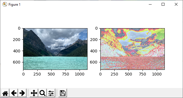
# Import the required libraries import PIL # Import the Python Imaging Library (PIL) from PIL import Image # Import the Image module from PIL from matplotlib import pyplot # Import the pyplot module from matplotlib from numpy import asarray # Import the asarray function from numpy
# Open the image file img = Image.open('Scene_01.png')
# Convert image to numpy array imgAry = asarray(img)
# Crop the array # Crop the array by selecting rows from 400 to 498 and columns from 300 to 398 imgAryCropped = imgAry[400:499, 300:399]
# Convert the cropped array back to an image mImg = Image.fromarray(imgAryCropped) # Create a new image from the cropped array
# Plot the original and cropped images pyplot.subplot(1, 2, 1) pyplot.imshow(img)
pyplot.subplot(1, 2, 2) pyplot.imshow(mImg)
# Show the plot pyplot.show() |
|
|
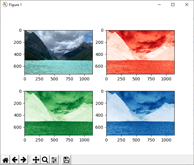
Splitting Image into Color Channels
|
# Import the required libraries import PIL from PIL import Image from matplotlib import pyplot from numpy import asarray
# Open the image file img = Image.open('Scene_01.png') #
# Convert image to numpy array imgAry = asarray(img)
# Print the array size and shape print('Size = ', imgAry.size, ',shape=', imgAry.shape) dim = imgAry.shape # Store the dimensions of the array
# Extract each color channel from the array imgAryCroppedCh1 = imgAry[0:dim[0], 0:dim[1], 0] # Extract the red channel imgAryCroppedCh2 = imgAry[0:dim[0], 0:dim[1], 1] # Extract the green channel imgAryCroppedCh3 = imgAry[0:dim[0], 0:dim[1], 2] # Extract the blue channel
# Convert the extracted color channels back to images mImgCh1 = Image.fromarray(imgAryCroppedCh1) # Create an image from the red channel array mImgCh2 = Image.fromarray(imgAryCroppedCh2) # Create an image from the green channel array mImgCh3 = Image.fromarray(imgAryCroppedCh3) # Create an image from the blue channel array
# Plot the original image and the extracted color channels pyplot.subplot(2, 2, 1) pyplot.imshow(img)
pyplot.subplot(2, 2, 2) pyplot.imshow(mImgCh1, cmap='Reds')
pyplot.subplot(2, 2, 3) pyplot.imshow(mImgCh2, cmap='Greens')
pyplot.subplot(2, 2, 4) pyplot.imshow(mImgCh3, cmap='Blues')
# Show the plot pyplot.show() |
|
|
|
import PIL from PIL import Image from matplotlib import pyplot
img = Image.open('Scene_01.png')
img.save('Scene_01.bmp', format='bmp') |
|
|
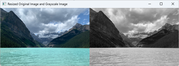
Converting Image to Gray Scale (OpenCV)
|
import cv2 import numpy as np
# Read an image from a file image = cv2.imread('Scene_01.png')
# Calculate the scaling factor so that the total width of the two images is 700 pixels scaling_factor = 700 / (2 * image.shape[1])
# Resize the original image resized_image = cv2.resize(image, None, fx=scaling_factor, fy=scaling_factor, interpolation=cv2.INTER_AREA)
# Convert the image to grayscale gray_image = cv2.cvtColor(resized_image, cv2.COLOR_BGR2GRAY)
# Convert the grayscale image back to BGR color space for concatenation gray_image_bgr = cv2.cvtColor(gray_image, cv2.COLOR_GRAY2BGR)
# Concatenate the resized original image and the resized grayscale image horizontally concatenated_image = np.hstack((resized_image, gray_image_bgr))
# Display the concatenated image in a window cv2.imshow('Resized Original Image and Grayscale Image', concatenated_image)
# Wait for a key press and close the window cv2.waitKey(0) cv2.destroyAllWindows() |
|
|
|
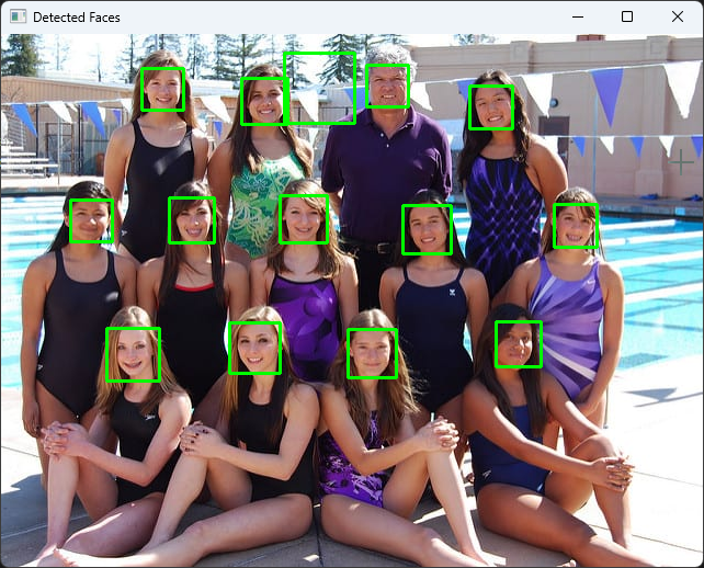
import cv2
# Load the pre-trained Haar Cascade classifier for face detection # this xml file can be downloaded at # https://github.com/opencv/opencv/blob/master/data/haarcascades/haarcascade_frontalface_default.xml face_cascade = cv2.CascadeClassifier('haarcascade_frontalface_default.xml')
# Read an image from a file # This test image was downloaded at How to Perform Face Detection with Deep Learning image = cv2.imread('SwimTeam.jpg')
# Convert the image to grayscale gray_image = cv2.cvtColor(image, cv2.COLOR_BGR2GRAY)
# Detect faces in the grayscale image using the Haar Cascade classifier faces = face_cascade.detectMultiScale(gray_image, scaleFactor=1.02, minNeighbors=15, minSize=(30, 30))
# Draw rectangles around the detected faces for (x, y, w, h) in faces: cv2.rectangle(image, (x, y), (x + w, y + h), (0, 255, 0), 2)
# Display the image with detected faces cv2.imshow('Detected Faces', image)
# Wait for a key press and close the window cv2.waitKey(0) cv2.destroyAllWindows() |
|
|
Reference
- How to Perform Face Detection with Deep Learning - Machine Learning Mastery (2019)