Laplace transform is one of the important sections of any Engineering Mathematics course. But if you don't understand what Laplace transform is and how it helps us to solve many engineering problems, it would just seem to you as one of the many things that seems to be designed just to make your school life difficult and miserable -:).

I'll build this page in four parts. The first part answers what the transform is, why engineers use it and when it works. The second part is the transform table, a graphical view of a function of s, and two worked examples. The third part turns a differential equation into a transfer function and models simple mechanical elements with it. The last part converts a transfer function into a state space matrix.

• What is Laplace Transform ?
• Why Laplace Transform ?
• Can we use Laplace Transform for Any kind of Differential Equation ?
• Do I always have to use Laplace Transform to solve a Differntial Equation ?
• Laplace Transform Table
• Graphical Representation of Laplacian Form
• Examples
• Example 1 : y'(t) + y(t) = u(t), y(0) = 0
• Example 2 : y''(t) + 2 y'(t) + 5 y(t) = sin(3 t), y(0) = 1  y'(0) = -1
• Transfer Function
• Transfer Function of Mechanical Systems - Modeling Mechnical System in Laplace Form
• Spring
• Damper
• Mass
• Spring-Mass
• Spring-Damper
• Spring-Mass-Damper
• Tortion Bar
• Tortion Damper
• Rotational Inertia
• Transfer Function to State Space Matrix

What is Laplace Transform ?

What is Laplace transform ? The mathematical definition of the Laplace transform is as follows. Don't get disappointed even if you don't understand the real meaning of this transform. I put this mathematical definition as a kind of cheatsheet in case when you may feel like looking at this and trying to draw any possible meaning out of this definition.

Just as a small hints for your future trial : You are looking at the two very important components of engineering math that I dealt in my side. One of the component you see is "Sum of Times" and the other component is "Exponential" form. If you dig further into Laplace Transform, you would learn the laplace variable 's' is complex number. Now you see another very important component of Mathematics which is 'complex number'. Just give it a try to understand the meaning of this transformation from what you intuitively understood from the section of 'Sum of Times', 'exponential form', 'complex numbers'.

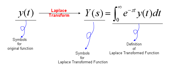
Let's read the definition term by term. The variable s is a complex number, s = σ + jω. So e^-st = e^-σte^-jωt does two jobs. The factor e^-jωt picks out the frequency ω, the same way the Fourier transform does. The factor e^-σt is a decaying weight, and it keeps the integral finite even for a y(t) that does not decay by itself.

A short calculation shows how the table entries come from the definition. For y(t) = 1, the integral of e^-st from 0 to infinity is 1/s, as long as the real part of s is positive. For y(t) = e^-at, the same integral gives 1/(s + a) when the real part of s is larger than -a. These two results are the u(t) and e^-at rows of the table further down.

The most important property is what happens to a derivative. Integration by parts turns the transform of y'(t) into sY(s) - y(0). So differentiation in t becomes multiplication by s, and the initial value enters as a constant. This single rule is the reason the transform turns a differential equation into an algebraic one.

• s is a complex frequency : Its imaginary part is the frequency ω, and its real part is a decay that keeps the integral finite.
• The integral starts at t = 0 : The transform only uses y(t) for t >= 0, so the initial values y(0) and y'(0) appear as separate terms.
• A derivative becomes a multiplication by s : The rule y'(t) to sY(s) - y(0) is the one every later section relies on.

Why Laplace Transform ?

Probably this section would be more important to most of the readers than the mathematical definition of the Laplace Transform. The definition tells you what the transform computes. This section tells you what it is good for, and the short answer is that it turns calculus into algebra.

My understanding (or many other understandings from other text books) would be as follows. As I mentioned in many other pages, the start point of using mathematics in engineering is to describe a real world problem into various mathematical forms. One of the mathematical forms that is most commonly used would be "Differntial Equation". As you may feel if you did Modeling using Differential Equations, you would have felt "Differential Equation would be an handy tool for DESCRIBING the real life problems, but not that easy to FIND SOLUTION from it".

Laplace Transform can be a very handy tools to help you FIND SOLUTION from a differential equation. If you transform a differential equation into a Laplace form, the transformed form became an Algebraic form from which even a junior high school student can get the solution. Simply put, Laplace Transform is a mathematical tool that can convert various differential equations into a form that even a junior high school student can solve.

Once you get the solution using the Laplace Transform, you normally have to go through "Inverse Laplace Transform" to express the solution in more meaningful format in the real life problem.

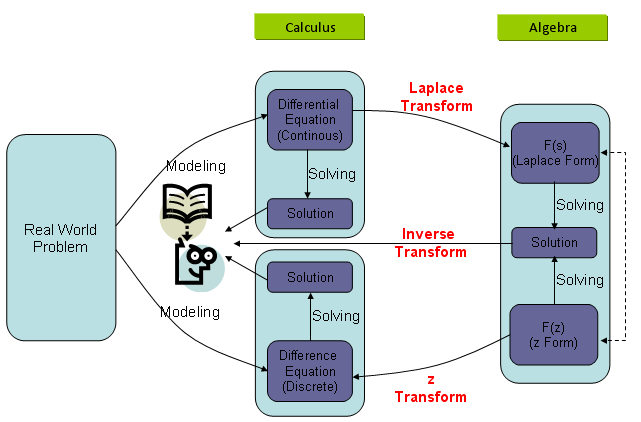
This overal process of how Laplace transform is being used can be illustrated as follows. I put three different diagram as follows.

First, many of our real life problems are described in the form of Differential Equations. You can use any kind of "Solution Process" to solve the differential equations.

As I mentioned, Laplace Transform is only a kind of "Solution Process" for a differential equation illustrated as below. (For now, let's ignore of 'z-transform' part.)

Following is just a simplified form of illustration shown above. Of course, you can draw you own diagram based on your own understanding.

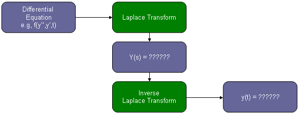
The price of the shortcut is the inverse transform at the end. In practice you rarely compute it from an integral. Instead you rewrite Y(s) as a sum of simple fractions and read each one back from the table, which is exactly what the Examples section does.

• Laplace Transform is one Solution Process among several : It replaces calculus with algebra, and it does not change the answer.
• The round trip has three steps : Transform the equation, solve for Y(s), and transform the result back to y(t).
• The z-transform plays the same role for difference equations : The concept diagram shows it as the discrete time counterpart of the Laplace Transform.

Can we use Laplace Transform for Any kind of Differential Equation ?

What do you think the answer is ? Unfortunately the answer is "No". Laplace Transform cannot be a solution for any kind of differntial solution. The form of Differential Equation you can solve using Laplace Transform is "Linear Differential Equation".

To be more precise, the method works best for linear differential equations with constant coefficients, such as y'' + 2y' + 5y = sin(3t). The reason is linearity. The transform of a sum is the sum of the transforms, and the transform of a constant times y is that constant times Y(s). So each term of the equation can be transformed on its own.

The method breaks down in two ways. The first is a nonlinear term. The transform of y² is not Y(s)², and no table entry gives it in terms of Y(s). The second is a coefficient that depends on t. The transform of t y(t) is -dY/ds, so an equation such as t y'' + y = 0 turns into another differential equation in s. That is sometimes useful, but it no longer gives a simple algebraic equation.

A nonlinear system can still use the transform after linearization around an operating point. This is the usual approach in control engineering.

• Linear with constant coefficients is the target : Every term then maps to a table entry multiplied by a constant.
• A nonlinear term has no Laplace form in terms of Y(s) : Terms such as y² or sin(y) block the method.
• A coefficient that depends on t gives a derivative in s : The equation stays a differential equation, so the method loses its advantage.

Do I always have to use Laplace Transform to solve a Differntial Equation ?

There is nothing "MUST" with this. As I mentioned, Laplace Transform is invented to HELP you to solve a problem. If you don't feel it is not helping you at all. You can just stick to whatever you would think is easy for you. As a matter of fact, in many text book example (the examples even in this page) they shows pretty simple differential equations for Laplace Transform. For these examples, you may get the feeling "Why do I have to go through this additional process.. I already know the solution for this differential equation without using Laplace Transform". I agree, at least I would have the same feeling as yours for most of the textbook example problems.

But there are many cases where it became easier to Lapalace Transform than trying to solve the differential equations as it is.

The transform helps most in three typical cases. The first is an input that switches on or jumps, such as a step, a delayed step u(t - α) or an impulse. The table handles these directly, while the classical method has to solve each time interval separately. The second is a set of coupled equations. Each one becomes an algebraic equation, and you solve the set like simultaneous equations. The third is a problem with given initial values, because y(0) and y'(0) enter automatically in the first step.

The transform also gives the transfer function. So even when you can solve one equation faster by hand, the Laplace form is the one that the later sections of this page and most of control engineering work with.

• Nothing forces you to use it : It is a tool, and the answer is the same whichever method you use.
• Switching inputs and coupled equations favour it : Steps, delays and impulses are single table entries in the s domain.
• Initial values come in automatically : The term sY(s) - y(0) carries them into the algebra at the first step.

Laplace Transform Table

We already saw the mathematical definition of the Laplace transform at the beginning of this page, but it is not easy to solve a differential equation purely based on the definition of the Lapalce Transform. If it is the case, you would not use Laplace Transform because the transformation process would be thought more complicated than solving the differential equation as it is. Fortunately, many mathemticians and engineers have done a lot of research and found the laplace form of expression for almost any components we see in various differential equation. Following is a table showing the laplace form of many mathematical components we normally see in various differential equation. I would say this is a kind of minimum sized table. You would see much longer table from various text book or many other sources you can google.

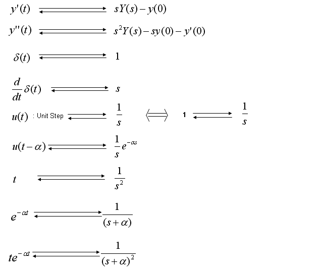
Performing the Laplace Transform is like a translating a sentence from a language to another language. When you have a differential equation, just split (or rewrite) the original differential equations into a set of small forms (words). And find the laplace form from the table (a kind of dictionary) corresponding components of the original equation. Look at the example at the end of this page or the examples from your text books.

Two rules let you read far more out of this short table. The first is linearity. The transform of a f(t) + b g(t) is a F(s) + b G(s), so you can transform an equation term by term. The second is the shift rule. Multiplying by e^-at in time replaces s with s + a in the Laplace form. That is why cos(wt) and e^-at cos(wt) have the same shape of transform, with s + a in place of s.

A third rule is the time delay. A function that is delayed by α and switched on at t = α gets an extra factor e^-αs. The u(t - α) row of the table is this rule applied to the unit step.

• Read the table in both directions : The same row gives the forward transform in Step 1 and the inverse transform in Step 4 of the examples.
• Linearity splits an equation into table entries : Each term is transformed on its own and the results are added.
• The shift rule doubles the table : e^-at times f(t) becomes F(s + a), which gives the damped rows from the undamped ones.

Graphical Representation of Laplacian Form

In many cases, you would get as a result of modeling your system (e.g, Transfer function of a Control System, Filter etc) a polynomials or rational functions of the laplace parameter 's'.

Except that unfamilar character 's', those polynomial and rational equations would be very similar to what you saw in your junior/senior high school math. But the interpretation of those equations would not be as straightforward/simple as it was with those equations in your high school math.

The difficulties come from the fact that the one you saw in high school math is using a real number and the equations with laplace parameter is using complex number. We haven't been trained much about plotting a function with complex variable. Even calculation of the equation is not easy and almost impossible to calculate those plotting points by hand.

But you don't have to worry about the calculation and even plotting the result since there are many softwares with which you can do this (e.g, Matlab/Octave, Mathematica, Maple etc).

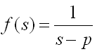
As the first example, let's assume that you have the following function. This is a complex function in which the independent variable "s" is a complex number.

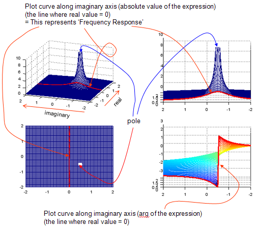
I would not explain much about how these plots are drawn since it would be better for you to work through the Matlab/Octave source code following the plot. (I intentionally does not try to use any complicated programming component and tried to write the script as much straightforward as possible. In terms of programming, it may not be an efficient code, but I try to make it more readable with minimum knowledge of the language.)

In this example, the variable a1 and b1 in the script is the two components of constituting the constant -p in the following equation. The script computes 1 ./ (s .+ p1), so p1 = a1 + b1 j stands for -p. Try change a1 and b1 in various values and see how these plot changes.

Just quick question assuming that you already played with the script and had some intuitive understanding of the following function. How the constant 'p' affect the result of the function ?

Maybe my question is not so clear. I didn't know example how I should ask. Have you noticed that the 'p' is the point where the result (magnitude) of this function (dependent variable) become very large (infinite number) ? If you noticed this, I think you have proper understanding of this function.

The thick redline in the graph has also very important meaning. It is the points where only imaginary component of 's' exists, no real part. The imaginary part of 's' is converted to be 'jw', where 'w' represents 'frequency'. Therefore, this thick red line represents the frequency response of the function.

 

re = -2:.05:2; im = -2:.05:2;

a1 = -0.5;

b1 = 0.5;

 

[X,Y] = meshgrid(re,im);

s = (X + Y*j);

s_jw = (0 + Y*j);

p1 = a1 + b1*j;

Zabs = abs(1 ./ (s .+ p1 ));

Zarg = arg(1 ./ (s .+ p1 ));

Zw = abs(1 ./ (s_jw .+ p1));

Zwarg = arg(1 ./ (s_jw .+ p1));

 

zmax = 10;

subplot(2,2,1); mesh(X,Y,Zabs);axis([re(1) re(end) im(1) im(end) 0 zmax]);

hold on;

plot3(X.*0,Y,Zw, 'linewidth',3,'color','r');

hold off;

view(-70,30);

 

subplot(2,2,2); mesh(X,Y,Zabs);axis([0 re(end) im(1) im(end) 0 zmax]);

hold on;

plot3(X.*0,Y,Zw, 'linewidth',3,'color','r');

hold off;

view(-90,10);

 

subplot(2,2,3); mesh(X,Y,Zabs);axis([re(1) re(end) im(1) im(end) 0 zmax]);

hold on;

plot3(X.*0,Y,Zw, 'linewidth',3,'color','r');

hold off;

view(0,90);

 

subplot(2,2,4); mesh(X,Y,Zarg);axis([0 re(end) im(1) im(end) -pi pi]);

hold on;

plot3(X.*0,Y,Zwarg, 'linewidth',3,'color','r');

hold off;

view(-90,10);

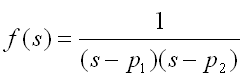
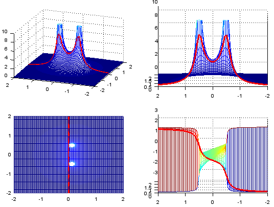
Next example is plotting the following function. In this function, you will get two points where the magnitude of the function become infinite. We say "This function has two poles".

See how the plot changes when you change a1,b1 and a2,b2. Especially how the shape of the thick red line changes as you change the values.

 

re = -2:.05:2; im = -2:.05:2;

a1 = -0.125;

b1 = 0.5;

a2 = -0.125;

b2 = -0.5;

 

[X,Y] = meshgrid(re,im);

s = (X + Y*j);

s_jw = (0 + Y*j);

p1 = a1 + b1*j;

p2 = a2 + b2*j;

Zabs = abs(1 ./ ((s .+ p1) .* (s .+ p2)) );

Zarg = arg(1 ./ ((s .+ p1) .* (s .+ p2)) );

Zw = abs(1 ./ ((s_jw .+ p1).*(s_jw .+ p2)) );

Zwarg = arg(1 ./ ((s_jw .+ p1).*(s_jw .+ p2)) );

 

zmax = 10;

subplot(2,2,1); mesh(X,Y,Zabs);axis([re(1) re(end) im(1) im(end) 0 zmax]);

        hold on;

        plot3(X.*0,Y,Zw, 'linewidth',3,'color','r');

        hold off;

        view(-70,30);

subplot(2,2,2); mesh(X,Y,Zabs);axis([0 re(end) im(1) im(end) 0 zmax]);

        hold on;

        plot3(X.*0,Y,Zw, 'linewidth',3,'color','r');

        hold off;

        view(-90,10);

subplot(2,2,3); mesh(X,Y,Zabs);axis([re(1) re(end) im(1) im(end) 0 zmax]);

        hold on;

        plot3(X.*0,Y,Zw, 'linewidth',3,'color','r');

        hold off;

        view(0,90);

subplot(2,2,4); mesh(X,Y,Zarg);axis([0 re(end) im(1) im(end) -pi pi]);

        hold on;

        plot3(X.*0,Y,Zwarg, 'linewidth',3,'color','r');

        hold off;

        view(-90,10);

Following is more general form. You would notice that numerator is not "1" any more. p1,p2 is the points called 'poles' where the result (magnitude) of the function goes infinite and z1,z2 is the points called 'zeros' where the result (magnitude) of the function goes to 0. But in this type of graph, the points for zeros would not be outstanding (You will see how to improve these in following example).

 

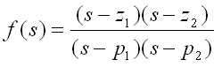
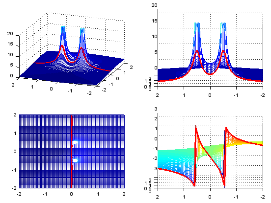
re = -2:.05:2; im = -2:.05:2;

p_a1 = -0.125;

p_b1 = 0.5;

p_a2 = -0.125;

p_b2 = -0.5;

z_a1 = 0.5;

z_b1 = 0.0;

z_a2 = 2.0;

z_b2 = 0.0;

 

[X,Y] = meshgrid(re,im);

s = (X + Y*j);

s_jw = (0 + Y*j);

p1 = p_a1 + p_b1*j;

p2 = p_a2 + p_b2*j;

z1 = z_a1 + z_b1*j;

z2 = z_a2 + z_b2*j;

 

Zabs = abs(((s .+ z1) .* (s .+ z2)) ./ ((s .+ p1) .* (s .+ p2)) );

Zarg = arg(((s .+ z1) .* (s .+ z2)) ./ ((s .+ p1) .* (s .+ p2)) );

Zw = abs(((s_jw .+ z1) .* (s_jw .+ z2)) ./ ((s_jw .+ p1) .* (s_jw .+ p2)) );

Zwarg = arg(((s_jw .+ z1) .* (s_jw .+ z2)) ./ ((s_jw .+ p1) .* (s_jw .+ p2)) );

 

zmax = 20;

subplot(2,2,1); mesh(X,Y,Zabs);axis([re(1) re(end) im(1) im(end) 0 zmax]);

hold on;

plot3(X.*0,Y,Zw, 'linewidth',3,'color','r');

hold off;

view(-70,30);

 

subplot(2,2,2); mesh(X,Y,Zabs);axis([0 re(end) im(1) im(end) 0 zmax]);

hold on;

plot3(X.*0,Y,Zw, 'linewidth',3,'color','r');

hold off;

view(-90,10);

 

subplot(2,2,3); mesh(X,Y,Zabs);axis([re(1) re(end) im(1) im(end) 0 zmax]);

hold on;

plot3(X.*0,Y,Zw, 'linewidth',3,'color','r');

hold off;

view(0,90);

 

subplot(2,2,4); mesh(X,Y,Zarg);axis([0 re(end) im(1) im(end) -pi pi]);

hold on;

plot3(X.*0,Y,Zwarg, 'linewidth',3,'color','r');

hold off;

view(-90,10);

The simplest way to make both Zeros and Poles outstanding is just to plot it in log scale as follows.

 

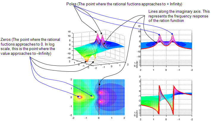
re = -2:.05:2; im = -2:.05:2;

p_a1 = -0.125;

p_b1 = 0.5;

p_a2 = -0.125;

p_b2 = -0.5;

z_a1 = 0.5;

z_b1 = 0.0;

z_a2 = 1.5;

z_b2 = 0.0;

 

[X,Y] = meshgrid(re,im);

s = (X + Y*j);

s_jw = (0 + Y*j);

p1 = p_a1 + p_b1*j;

p2 = p_a2 + p_b2*j;

z1 = z_a1 + z_b1*j;

z2 = z_a2 + z_b2*j;

 

Zabs = abs(((s .+ z1) .* (s .+ z2)) ./ ((s .+ p1) .* (s .+ p2)) );

Zabs = 10 * log10(Zabs);

Zarg = arg(((s .+ z1) .* (s .+ z2)) ./ ((s .+ p1) .* (s .+ p2)) );

Zw = abs(((s_jw .+ z1) .* (s_jw .+ z2)) ./ ((s_jw .+ p1) .* (s_jw .+ p2)) );

Zw = 10 * log10(Zw);

Zwarg = arg(((s_jw .+ z1) .* (s_jw .+ z2)) ./ ((s_jw .+ p1) .* (s_jw .+ p2)) );

 

zmax = 15;

 

subplot(2,2,1); mesh(X,Y,Zabs);axis([re(1) re(end) im(1) im(end) -zmax zmax]);

hold on;

plot3(X.*0,Y,Zw, 'linewidth',3,'color','r');

hold off;

view(-30,15);

caxis([-zmax zmax]);

colormap(hsv(20));

 

subplot(2,2,2); mesh(X,Y,Zabs);axis([0 re(end) im(1) im(end) -zmax zmax]);

hold on;

plot3(X.*0,Y,Zw, 'linewidth',3,'color','r');

hold off;

view(-90,10);

caxis([-zmax zmax]);

colormap(hsv(20));

 

subplot(2,2,3); mesh(X,Y,Zabs);axis([re(1) re(end) im(1) im(end) -zmax zmax]);

hold on;

plot3(X.*0,Y,Zw, 'linewidth',3,'color','r');

hold off;

view(0,90);

caxis([-zmax zmax]);

colormap(hsv(20));

 

subplot(2,2,4); mesh(X,Y,Zarg);axis([0 re(end) im(1) im(end) -pi pi]);

hold on;

plot3(X.*0,Y,Zwarg, 'linewidth',3,'color','r');

hold off;

view(-90,10);

Let's connect the plots to the scripts. The equations are written with s - p, but the scripts compute s .+ p1. So the pole of the first plot sits at s = -p1 = 0.5 - 0.5j, and that is where the peak appears in the top view. In the same way, the zeros of the last two plots sit on the negative real axis, at s = -0.5 and at s = -2 or s = -1.5.

The poles in the other three scripts are at s = 0.125 +/- 0.5j. Their real part is positive, so they lie to the right of the red line. A pole on that side means that the time response grows without limit, so the system is unstable. For a stable system, every pole lies to the left of the imaginary axis. The red frequency response curve shows peaks near ω = +/-0.5, the imaginary parts of the poles. A pole closer to the imaginary axis gives a taller and sharper peak.

The scripts are Octave code. MATLAB does not accept the .+ operator or the arg function, so write + and angle there. Newer Octave releases have also dropped .+.

• A pole is where the magnitude goes to infinity : For 1/(s - p) it is the point s = p.
• A zero is where the magnitude goes to 0 : The log scale plot shows the zeros as deep valleys.
• The imaginary axis carries the frequency response : A pole close to it produces a peak at its own frequency.
• Poles must lie on the left for stability : The example poles at 0.125 +/- 0.5j lie on the right, so that system is unstable.

Examples

Both examples use the same five steps. Step 1 transforms each term with the table, Step 2 and Step 3 solve for Y(s), and Step 4 and Step 5 break Y(s) into table entries and transform back. Example 1 is a first order equation with a step input. Example 2 is a second order equation with a sinusoidal input and nonzero initial values.

Example 1 : y'(t) + y(t) = u(t), y(0) = 0

Example 1 is a first order system that starts at rest and receives a unit step at t = 0. Before solving it, predict the answer. The output should start at 0 and settle at 1, because y' is 0 in the steady state and the equation then says y = 1.

Step 1 : Find Laplace form for each terms of the equation from Laplace Transform Table

y'(t) ---> s Y(s) - y(0) = s Y(s) because we defined y(0) = 0 in this example

y(t) --> Y(s), this is definition of Laplace Transform

u(t) --> 1/s, u(t) means the unit step function.

Step 2 : Plug the result of step 1 into the original equation

s Y(s) + Y(s) = 1/s

Step 3 : Rearrange the result of step 2 in the form of Y(s) = ????

Y(s)(s+1) = 1/s

Y(s) = (1/s)/(s+1) = 1/s(s+1)

Step 4 : Find the inverse Transform for the result of Step 3 from Laplace Transform Table

i) Did you find any mapping table for 1/s(s+1) ?

ii) No

iii) Then try to break down 1/s(s+1) into a form which has a mapping table.

: this is the most tricky part, and you would need some algebraic skills. If you convert this as follows ...

Y(s) = 1/s - 1/(s+1)

From the table, you would get the following mapping

1/s ---> 1

1/(s+1) --> e^(-t)

Step 5 : Convert Y(s) = 1/s - 1/(s+1) into y(t) form using the result of step 4.

y(t) = 1 - e^(-t)

The partial fractions in Step 4 are 1/s - 1/(s+1), with a minus sign. You can check them by putting the two fractions over a common denominator: (s + 1 - s)/s(s+1) = 1/s(s+1). The minus sign is also what gives y(t) = 1 - e^-t. This result meets both predictions. It starts at y(0) = 0, and y' + y = e^-t + 1 - e^-t = 1 for every t > 0.

Example 2 : y''(t) + 2 y'(t) + 5 y(t) = sin(3 t), y(0) = 1  y'(0) = -1

Example 2 adds three complications at once. The equation is second order, the input is a sinusoid, and both initial values are nonzero. Watch how the initial values enter in Step 1 and stay in the algebra until the end.

Step 1 : Find Laplace form for each terms of the equation from Laplace Transform Table

y''(t) ---> s^2 Y(s) - s y(0) - y'(0) ---> s^2 Y(s) -s (1) - (-1) ---> s^2 Y(s) - s + 1

              because we defined y(0) = 1  y'(0) = -1 in this example

y'(t) ---> s Y(s) - y(0) = s Y(s) - 1 because we defined y(0) = 1 in this example

y(t) --> Y(s), this is definition of Laplace Transform

sin(3 t) --> 3/(s^2+9)

Step 2 : Plug the result of step 1 into the original equation

      (s^2 Y(s) - s + 1) + 2(s Y(s) - 1) + 5 Y(s) = 3/(s^2+9)

Step 3 : Rearrange the result of step 2 in the form of Y(s) = ????

(s^2 Y(s) - s + 1) + 2(s Y(s) - 1) + 5 Y(s) = 3/(s^2+9)

==> s^2 Y(s) - s + 1 + 2 s Y(s) - 2 + 5 Y(s) = 3/(s^2+9)

==> (s^2 + 2 s + 5) Y(s) -s - 1 = 3/(s^2+9)

==> (s^2 + 2 s + 5) Y(s) =  s + 1 + 3/(s^2+9)

==> Y(s) =  [s + 1 + 3/(s^2+9)]/(s^2 + 2 s + 5)

Step 4 : Find the inverse Transform for the result of Step 3 from Laplace Transform Table

i) Did you find any mapping table for [s + 1 + 3/(s^2+9)]/(s^2 + 2 s + 5) ?

ii) No

iii) Then try to break it down into a form which has a mapping table.

: this is the most tricky part, and you would need some algebraic skills. If you convert this as follows ...

Y(s) = (s+1)/(s^2 + 2 s + 5) + 3/[(s^2+9)(s^2 + 2 s + 5)]

 

Does (s+1)/(s^2 + 2 s + 5) have any mapping table ? It doesn't seem to have.. but if you rearrange as follows, you would see some mapping. (I know this is tricky..)

(s+1)/(s^2 + 2 s + 5) ---> (s+1)/((s+1)^2+4) --> e^-t cos(2t)

 

Does 3/[(s^2+9)(s^2 + 2 s + 5)] have any mapping table ? It doesn't seem to have..

But with some magic called 'partial decomposition technique', you can convert this as follows.

3/[(s^2+9)(s^2 + 2 s + 5)] --> 3/26[-(s+2)/(s^2+9) + (s+4)/(s^2+2s+5)]

Now you can break this even further

(s+2)/(s^2+9) --> s/(s^2+9) + 2/(s^2+9) --> cos(3t) + 2/3 sin(3t)

(s+4)/(s^2+2s+5) --> (s+1)/[(s+1)^2 + 4] + 3/[(s+1)^2 + 4]

                         --> e^-t cos(2t) + 3/2(e^-t sin(2t))

 

Step 5 : Convert Y(s) = (s+1)/((s+1)^2+4) + 3/26[-(s+2)/(s^2+9) + (s+4)/(s^2+2s+5)]

                       into y(t) form using the result of step 4.

y(t) = e^-t cos(2t) + 3/26[-cos(3t) - 2/3 sin(3t) + e^-t cos(2t) + 3/2(e^-t sin(2t))]

Two lines in this example need care. The first transform in Step 1 is s²Y(s) - s + 1. The other one is the inverse of 3/[(s+1)² + 4] in Step 4. The table row for e^-at sin(wt) is w/((s+a)² + w²), so with a = 1 and w = 2 the inverse is 3/2 e^-t sin(2t), not a cosine. The same correction applies to the last term of y(t) in Step 5.

Collecting the terms gives y(t) = 29/26 e^-t cos(2t) + 9/52 e^-t sin(2t) - 3/26 cos(3t) - 1/13 sin(3t). At t = 0 this is 29/26 - 3/26 = 1, and its derivative is -1, so both initial values match. The two e^-t terms are the transient, and they decay to zero. What remains is the steady state -3/26 cos(3t) - 1/13 sin(3t), a sinusoid at the input frequency 3.

• The five steps are the same for every linear equation : Only the algebra in Step 3 and the partial fractions in Step 4 get longer.
• Partial fractions are the step to check : Recombine the fractions over a common denominator before you transform them back.
• Transient and steady state separate in s : The roots of s² + 2s + 5 give the decaying terms, and the roots of s² + 9 from the input give the steady state.

Transfer Function

As you saw in previous sections, you can convert a differential equation into a laplacian form (s domain function) by applying the laplace transform table.

If this is a model for any real life system, it would have a special term representing 'Input' of the system and a term representing 'Output' of  the system. You can rearrange the equation in a form as follows and this form of equation is called 'Transfer Function'.

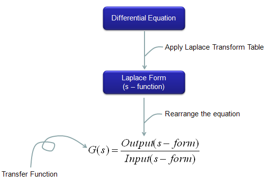
I think the widest application of Laplace form would be the analysis of this transfer function which means the analysis of the system that you modeled.

One condition is hidden in this definition. The transfer function assumes that all initial values are zero. Otherwise the terms y(0) and y'(0) would stay in the equation, and the ratio of output to input would depend on them.

Example 1 shows the idea. With zero initial values, y' + y = u becomes (s + 1)Y(s) = U(s). So G(s) = Y(s)/U(s) = 1/(s + 1). The output for any input is then Y(s) = G(s)U(s). For the unit step, U(s) = 1/s and Y(s) = 1/s(s+1), the same as in Example 1. The roots of the denominator of G(s) are the poles of the Graphical Representation section, so the transfer function also carries the stability of the system.

• G(s) is output over input : Both are in Laplace form, and every initial value is set to 0.
• The output is G(s) times the input : Multiplying in s replaces solving the equation again for each new input.
• The denominator holds the poles : Its roots decide the stability and the natural frequencies of the system.

Transfer Function of Mechanical Systems - Modeling Mechnical System in Laplace Form

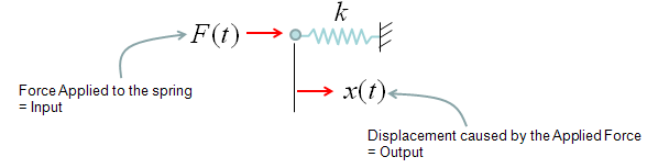
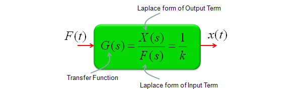
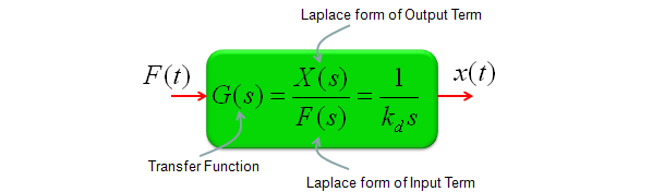
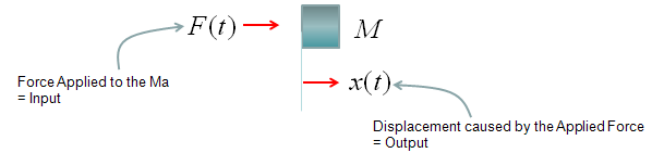
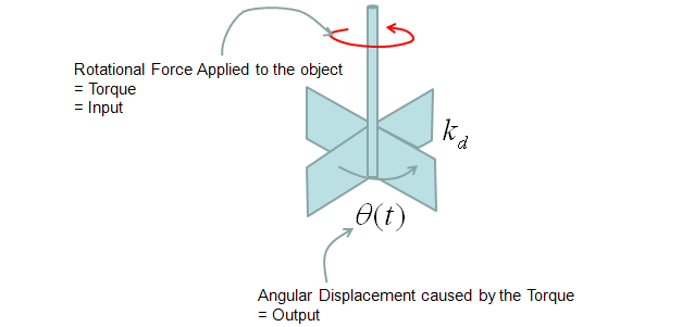
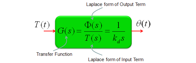
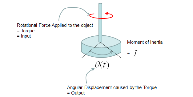
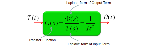
Every mechanical element below is modelled the same way, in three pictures. The first shows the element with its input, a force F(t) or a torque T(t), and its output, a displacement x(t) or an angle θ(t). The second writes the force balance and transforms it. The third is the transfer function block. The first six elements move in a line, and the last three rotate.

Spring

A spring pushes back in proportion to how far you stretch it, so F = kx. There is no derivative in this law. The transfer function is therefore the constant 1/k, and it does not depend on s.

Damper

A damper resists speed rather than position. Its force is k_d times the velocity dx/dt, so the Laplace form picks up one factor of s. The transfer function is 1/(k_ds).

Mass

A mass resists acceleration, so F = M d²x/dt². The second derivative gives s². The transfer function 1/(Ms²) therefore has a double pole at s = 0.

Spring-Mass

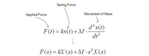
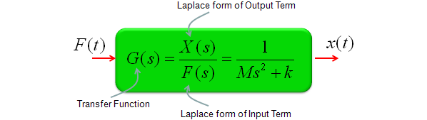
Now the spring and the mass share one displacement x(t). The applied force has to supply both the spring force and the force that accelerates the mass, so the two terms add. The transfer function is 1/(Ms² + k). Its poles at s = +/-j√(k/M) sit on the imaginary axis, so the mass oscillates at ω = √(k/M) without decaying.

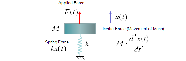
Spring-Damper

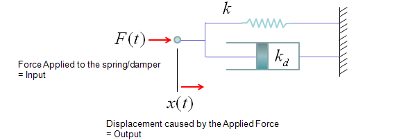
Here the spring and the damper sit in parallel between the force and the wall. They share the displacement x(t), so again the forces add. The transfer function 1/(k_ds + k) has one pole at s = -k/k_d. A step force therefore gives a displacement that rises smoothly to F/k without oscillating.

Spring-Mass-Damper

This is the standard second order system, and the force equation adds all three terms. The drawing places the damper between the mass and the force. But the equation applies the damper force k_ddx/dt to the mass itself, as if the damper were anchored to the wall like the spring. The transfer function below belongs to that anchored arrangement.

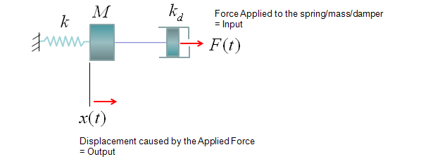
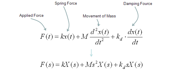
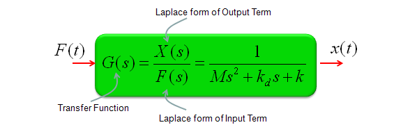
The damping decides the shape of the response. The poles are complex, and the response oscillates, when k_d² < 4Mk. They are real, and the response does not oscillate, when k_d² >= 4Mk.

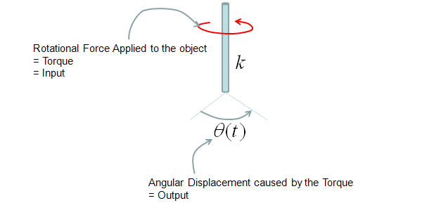
Tortion Bar

The rotational elements mirror the linear ones. Torque T(t) takes the place of force, and the angle θ(t) takes the place of displacement, with Φ(s) as its Laplace form. The Tortion Bar twists in proportion to the torque, so it is the rotational spring with transfer function 1/k.

Tortion Damper

The Tortion Damper is the rotational damper. Paddles that turn in a fluid give a torque proportional to the angular velocity dθ/dt. So the transfer function has one factor of s, 1/(k_ds).

Rotational Inertia

A disc with moment of inertia I resists angular acceleration, so T = I d²θ/dt². This is the rotational mass, and its transfer function is 1/(Is²).

The table below lines up the translational and rotational elements. Each pair has the same transfer function, with torque and angle in place of force and displacement.

• Each derivative becomes one power of s : A spring gives s⁰, a damper s¹ and a mass s².
• Elements that share one displacement add their terms : The spring, mass and damper together give the denominator Ms² + k_ds + k.
• Rotation mirrors translation : Torque, angle, torsional stiffness and moment of inertia take the places of force, displacement, stiffness and mass.

Transfer Function to State Space Matrix

There are many different ways of analyzing the transfer function. Graphical Representation of Laplacian Form is one of the method for the analysis and there are many other method as well. One of the other methods for the system transfer function would be to use 'State Matrix'.

A transfer function is normally represented in the form as follows. (If you don't have the form exactly expressed in this form, you would be able to rearrange it to this form without much difficulties)

The State Matrix of a system has the following format.

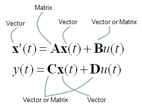
The goal is to identify A,B,C,D matrix out of your transfer function and followings are those matrix extracted from the transfer function. Don't get scared too much. Once you get the transfer function as shown above, just pull out the coefficients of each term and place in the A,B,C,D matrix as shown below.

This may look like "Making a simple things into more complicated one" and you may think "Why do we have to do this kind of stupid things ?".

But it is not the case. There have been a lot of people who has done great jobs to extract many useful information from this State Space matrix equations. So, once you get these A,B,C,D , you can use a lot of tricks which is made for State-Space analysis to understande the properties of the the transfer function.

You can derive this State-Space matrix equation from differential equations (Please see here for the details)

This arrangement of the matrices is called the controllable canonical form. Two details in it need care. The first is the vector C. For the numerator s^m + a_m-1s^m-1 + ... + a₀, C has n entries. They are a₀ to a_m-1, then the leading coefficient 1 of s^m, then zeros. The picture leaves out that 1. The numerator also does not have to start with 1, because its leading coefficient simply goes into C.

The second detail is D = 0. It holds only when m < n. When m = n, divide the numerator by the denominator first, and the quotient becomes D.

Let's check it on T(s) = (s + 3)/(s² + 3s + 2), with n = 2 and m = 1. The coefficients are b₀ = 2, b₁ = 3 and a₀ = 3. So A = [0 1; -2 -3], B = [0; 1], C = [3 1] and D = 0. The eigenvalues of A are -1 and -2, the roots of s² + 3s + 2. They are the poles of T(s), so the state space form keeps the stability of the transfer function.

• The denominator fills the last row of A : Its coefficients appear with a minus sign, and the rows above it only shift the states.
• The numerator fills C : Include the leading coefficient of the numerator, and use D only when the degrees are equal.
• The eigenvalues of A are the poles : The state space form and the transfer function describe the same system.