Beam Forming
What is BeamForming ? It means just as it sounds. BeamForming is a techology to 'Form' a 'beam'.
Then what does it mean by 'beam' in this context ? I would say it means 'electromagnatic wave radiation pattern(propagation pattern) for a set of antenna system'. Simply put, BeamForming is a technic that constuct the antenna radation pattern pointing towards specific direction.
Before diving into the details, let me give you 'super simplified' principles of beamforming/beamsteering.
1. If you put multiple number of antenna with a certain distances, you will always have some special shape of beam which is different from the radiation pattern from single isotropic antenna.
2. if you want to have a specific shape of beam you need to put those multiple antenna in a specific distances between them ==> BeamForming
3. if you want to point the team toward a specific direction, you need to transmit the signal through each of the antenna elements with certain amount of phase difference. ==> BeamSteering
High level meaning is simple like this.. but real implementation would be very complicated and is out of my understanding. So I would just give you only a big picture of this technology.
- Motivation (Why we need BeamForming ?)
- High Level view of BeamForming Implementation - Mapping Function, Spatial Filter
- How to 'Form' a beam ?
- Technology for BeamForming
- Basic Concept : Array Antenna
- Charecterization of Array Antenna - Beam Pattern Plot
- Basic Concept : Beam Forming - Phased Array
- Modeling BeamForming
- Beamforming in LTE
- Precoding for BeamForming
- Single-layer random beamforming (Antenna port 5, 7, or 8) : 36.101 B.4.1
- Dual-layer random beamforming (antenna ports 7 and 8) : 36.101 B.4.2
- Generic beamforming model (antenna ports 7-14) : 36.101 B.4.3
- Example 1 : 8 x 2 (8 Antenna, 2 Layers)
- CSI RS Configuration
- Beamforming in 5G/NR (Massive MIMO)
Motivation (Why we need BeamForming ?)
Why we need beamforming ?
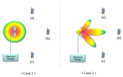
It is simple. Let's look at the two illustrations as shown below. There are two antenna system and let's assume that the two antenna is transmitting the exactly same amount of total energy.
In case 1, the antenna system is radiating the energy in almost same amount in all direction. The three UEs around the antenna would receive almost same amount of the energy but a large portions of energy not directed to those UEs is wasted.
In case 2, the signal strength of the radiation pattern ('beam') is specially 'formed' in such a way that the radiated energy in direction to UEs are much stroger than the other parts which is not directed to UEs.
High Level view of BeamForming Implementation - Mapping Function, Spatial Filter
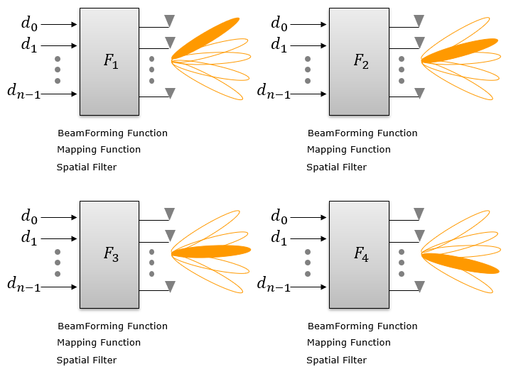
Very high level view on how to implement BeamForming can be illustrated as follows. It shows a set of data is going into a special function and the special function form a specific beam and transmit the data through the beam. The shape and direction of a beam is determined by what kind of function is used. This kind of special function is often called as BeamForming Function or Mapping Function or Spatial Filter. Applying the same Mapping function or Spatial Filter mean that it forms the same beam (i.e, same direction, same shape, same power of the beam).
Now the question is how these mapping function (or beamform algorithm) is implemented. The remaining of this page is all about the general logic of this mapping function. Simply put, the major component of the mapping functions are
-
Number of Antenna Elements in the array
-
Structure of Antenna Elements in the array
-
Phase and Amplitude applied to each of the data(signal) path => this can be done in software at the baseband or hardware(electrical circuit) at RF or mmWave frequency
By now, you would ask 'How can we form a beam ?'. If you want to understand this mechanism in pricise and clear way, you need to turn to the dry and boring mathematics. We will look into this mathematical way of explanation in following section(Basic Concept : Array Antenna), but before falling asleep with math, let's build up some intuitive understanding on the principles of the beam forming.
The basic principle of forming a beam is to use the property of interference of the multiple waves. If the multiple waves interfere each other at 'In-phase', the amplitude of the interfered waves gets bigger (this is called 'Constructive interference). If the multiple waves interfere each other at 'Out-of-phase', the amplitude of the interfered waves cancels each other(this is called destructive interference). If multipe waves propagating in 2D or 3D spaces, the resulting interference would show a specific pattern in which some part of the spaces shows constructive interference and some other parts shows desctructive interference. The part performing constructive interference form a beam pointing to a specific direction. Check out this slides(animation) and hope you can get some intuitive understanding.
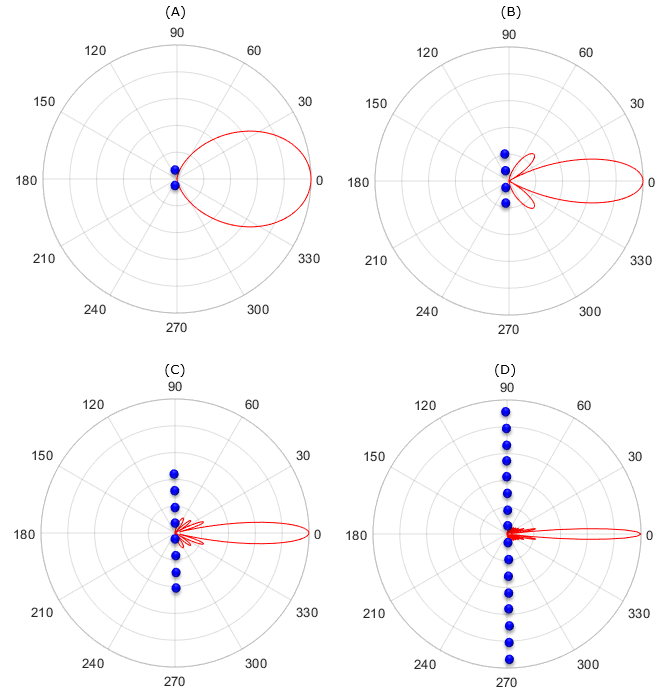
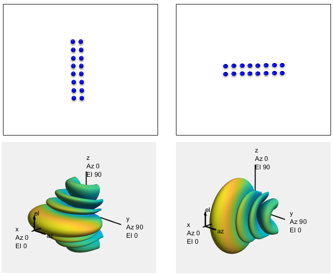
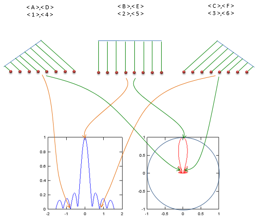
The simplest way of forming a beam is to put multiple antenna in an array. There are many different ways of aligning those antenna antenna elements, but one of the simplest way is to align the antenna along a line as shown in the following example. The intuitive idea you should see here is that you will get a sharper beam as you put more antenna elements in the array.
NOTE : This example plots were created by Matlab PhaseArrayAntenna toolbox and the source code for this example and more examples are posted here.
Also I have posted several pages in my visual note : www.freetechslide.com in the form of slideshow and animations of various antenna radiation pattern so that you can understand the radiation pattern for various antenna structure in more intuitive way. Check [Engineering]->[1]->[Antenna Radiation], [Array Antenna] in www.freetechslide.com
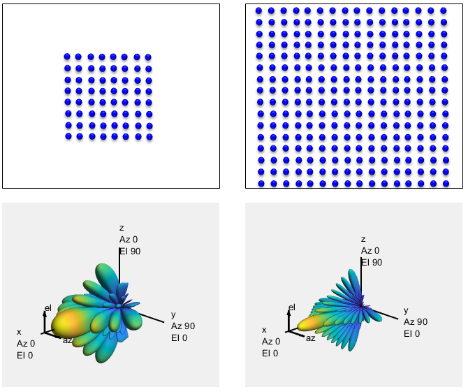
Another way of arranging the elements in an array is align the elements in a two dimensional sqaure as shown in the following examples. The intuitive idea you should see here is that you will get a sharper beam as you put more antenna elements in the array.
NOTE : This example plots were created by Matlab PhaseArrayAntenna toolbox and the source code for this example and more examples are posted here. For more diverse patterns for various different antenna array, I put more examples in my other notes. Try the pages at www.slide4math.com

Now let's think of another type of two dimensional array in which the shape of the array is not square as shown below. The intuition you can get is that the beam compressed more along the axis of more elements.
NOTE : This example plots were created by Matlab PhaseArrayAntenna toolbox and the source code for this example and more examples are posted here.
There are several different ways to implement the beamforming. Followings are couple of techniques most commonly used (As I mentioned, the details of implementation is out of my understanding).
For a little bit further details, see All Beamforming Solutions Are Not Equal. This is mainly for WLAN, but can be a good introduction.
Switched Array Antenna : This is the technique that change the beam pattern (radiation form) by switching on/off antenna selectively from the array of a antenna system.
DSP Based Phase Manipulation : This is the technique that change the beam pattern (radiation form) by changing the phase of the signal going through each antenna. Using DSP, you can change the signal phase for each antenna port differently to form a specific beam pattern that is best fit for one or multiple specific UEs.
Beamforming by Precoding : This is the technique that change the beam pattern (radiation form) by applying a specific precoding matrix. This is the technique used in LTE. In LTE, following transmission mode is implemeting 'BeamForming' implictely or explicitely.
-
TM 6 - Closed loop spatial multiplexing using a single transmission layer.
-
TM 7 - Beamforming (Antenna port 5)
-
TM 8 - Dual Layer Beamforming (Antenna ports 7 and 8)
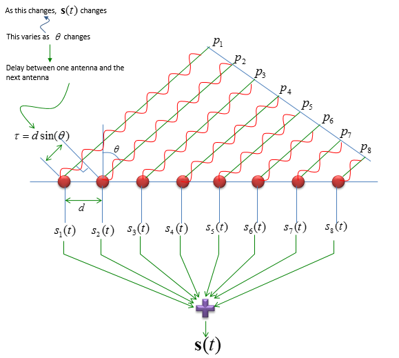
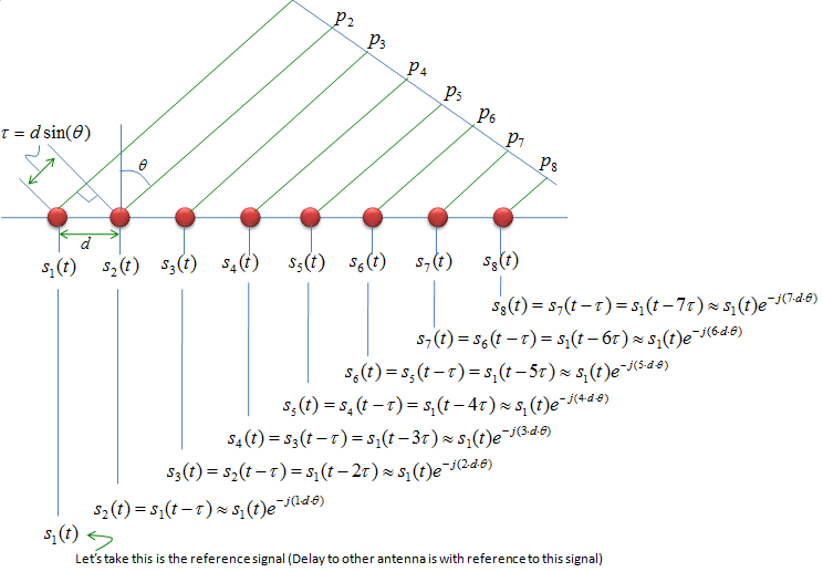
Since the BeamForming is mostly based on Array Antenna, let's take a look at the basic principles of Array Antenna. Let's suppose we have a antenna array in which each of the antenna is placed apart from each other with a certain distance (d). And then, suppose multiple rays of beam transmitted from a single source is received by each of the antenna in the array. If all the rays from the single source is coming directly (meaning theta in the following illustration is 0) into the antenna, there would be no differences in terms of distance along which each of the rays travelled from the source to each of the reciever antenna. So if you sum up the energy recieved by each antenna, it will be same as each of the wave sum up constructively. However, if the direction of the ray and the axis of antenna array is not in right angle (meaning the theta is not 0), the travel distance of each ray (p1,p2,..,p8) gets different and the difference can be expressed as d sin(theta) as shown in the following illustration.
Now let's describe what I explained above into mathematical expression. If I take the received signal at the first antenna (the leftmost antenna) as the reference antenna and the signal received at each of the antenna can be represented as follows. (This would the point where many people gave up further reading/study because of the math. But in most of engineering and science, there are many cases where you can never understand completely without a certain degree of math. So, don't give up just because of the math... and try to understand the meaning of each mathematica terms. When I am explaining about this array antenna, I first talked about the travel path difference and angle between antenna array axis and the beam ray hitting the antenna. In the mathematical expression, you still see the angle term 'theta', but you don't see any direct term that look like 'travel path'. Actually we don't know the exact travel difference of each beam because we don't know the exact location of the beam source. The only thing we know is the travel path difference between each beam hitting on each antenna. That travel path difference can be expressed as e^(-j * n * d * theta) where n is the index of the antenna being numbered 0 from the leftmost antenna. Keeping this in mind, take close loot at each mathematical expression and it would make sense to you. If you are not familiar with interpreting the meaining of e^(-theta), you may refer to complex number page).
Another way of visualizing this summation process would be as follows :
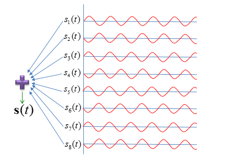
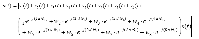
Now we formulated the signal coming into each antenna. Now let's formulate the signal that combined all the signal coming into each antenna. It is simple, you only have sum up all the signals comining into each antenna and it can be presented as follows.
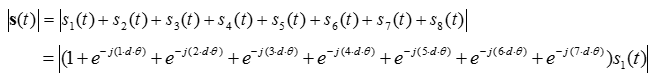
You can represent this equation into a vector notation as follows.(Many people even including me get intimidated when seeing this kind of matrix/vector expression. Don't get scared. We have already learned basic operations from high school or freshmen university math course. We just didn't have enough chance for enough practice. So if you get somehow uneasy feeling about this, just expand the following equation by hand and you will get more familiar expression as above. Doing this kind of practice whenever you see this kind of vector/matrix notation, gradually you will get more and more familiar and such an uneasy feeling would disappear. Nobody else can do this kind of practice for you)
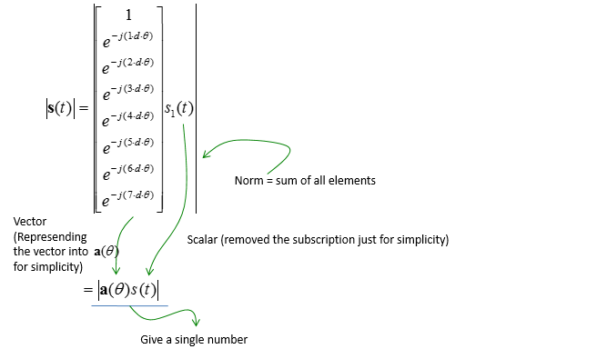
Note : I posted the graphical representation of this vector in my visual note www.freetechslide.com . Check [Engineering] -> [1] -> [Radiation Pattern]. You would see the effect of parameters like 'd' in more intuitive way in the visual note.
Charecterization of Array Antenna - Beam Pattern Plot
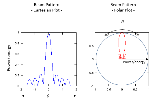
When you characterize (represent the performance of an Antenna array), you might have seen the types of plots as shown below. In some documents, you would see the plot like the one on the left and in some other document you would see the one on the right. Actually these two represents the exact the same thing. They just plot the same thing in two different coordinate system. The one on the left is the representation of (trancemitted or received power) vs angle in Cartesian coordinate and the right one is the representation of the same data in polar coordinate.
Power and Energy in the plot would be familiar to you. Then, what does the theta (angle) represents ? It is the angle between the direction of ray and the axis of antenna array. If reciever is the array antenna and the transmitter is a single transmitter far enough from the reciever antenna, the angle can be represented as follows. In this illustration, I set the distance (r) to be infinite to assume that the all the rays reaches the reciever antenna in paralelle. It reality, the distance cannot be infinite. it is just far enough to make the assumption meaningful. You can set the angle (theta) by placing the transmitter antenna to different location on the circumference (as in the top track) or by rotating the antenna array (as in the bottom track). In this case, you may think that the plots shown above reprents total power recieved by all the antenna on the array.
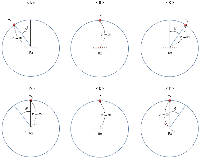
The same logic applies when the transmitter antenna is the array antenna and the reciever antenna is a point far away from the transmitter. The angle is the angle between the direction of ray and the axis of antenna array. The angle can be represented as follows. In this illustration, I set the distance (r) to be infinite to assume that the all the rays reaches the reciever antenna in paralelle. It reality, the distance cannot be infinite. it is just far enough to make the assumption meaningful. You can set the angle (theta) by placing the recieving antenna to different location on the circumference (as in the top track) or by rotating the antenna array (as in the bottom track). In this case, you may think that the plots shown above represents total power recieved by the reciever antenna.
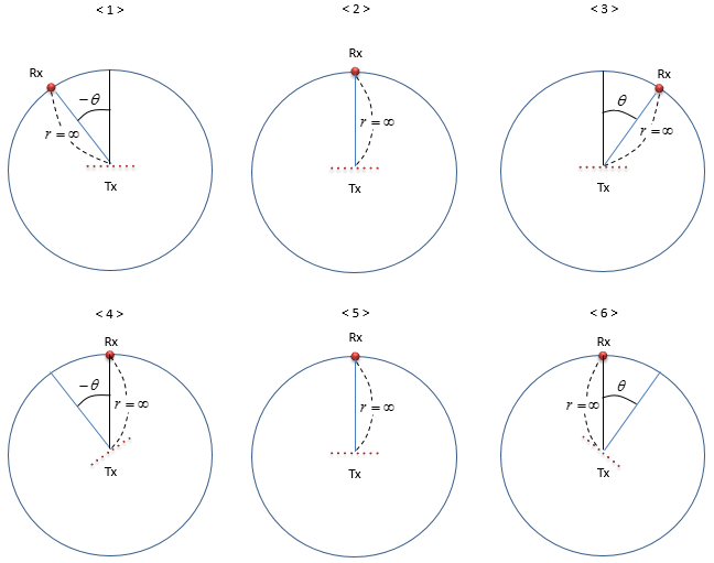
In above illustration, you have seen four different cases of representing the angle. Even though the function of the antenna array (being reciever or transmitter) is different and the way making the angle (by moving reciever/transmitter antenna by rotating the antenna array), the overall shape of the plot is same (at least in theory). The only difference would be the scale of Engergy/Power depending on whether it represents the reciever power or transmitter power. So if we ignoare the scale of the engery/power axis, you can interpret the graph (Power/energy vs theta) as shown below.
As you see here, the energy/power gets maximum when the angle (theta) is 0. To get the max energy when the angle is zero, the distance between one antenna in the array and another antenna next to it should be a half of wave length.
If you want to play with this graph, try running the follow matlab toy code.
theta = -0.5*pi:pi/100:0.5*pi;
d = 2.0;
a_theta = [exp(-j .* 0 .* d .* theta) ;
exp(-j .* 1 .* d .* theta);
exp(-j .* 2 .* d .* theta);
exp(-j .* 3 .* d .* theta);
exp(-j .* 4 .* d .* theta);
exp(-j .* 5 .* d .* theta);
exp(-j .* 6 .* d .* theta);
exp(-j .* 7 .* d .* theta)];
a_theta_sum = sum(a_theta);
a_theta_sum_abs = abs(a_theta_sum);
a_theta_sum_abs = a_theta_sum_abs ./ max(a_theta_sum_abs);
a_theta_sum_abs_dB = 10 .* log(a_theta_sum_abs);
for i = 1:length(a_theta_sum_abs_dB)
if a_theta_sum_abs_dB(i) <= -30
a_theta_sum_abs_dB(i) = -30;
end;
end;
a_theta_sum_abs_dB = a_theta_sum_abs_dB - min(a_theta_sum_abs_dB);
a_theta_sum_abs_dB = a_theta_sum_abs_dB/max(a_theta_sum_abs_dB);
subplot(2,2,1);plot(theta,a_theta_sum_abs);
xlim([-pi/2 pi/2]);
set(gca,'xtick',[-pi/2 -pi/4 0 pi/4 pi/2]);
set(gca,'xticklabel',{'-pi/2' '-pi/4' '0' 'pi/4' 'pi/2'});
subplot(2,2,2);polar(theta + 0.5*pi,a_theta_sum_abs,'-r');
t = findall(gcf,'type','text');
delete(t);
subplot(2,2,3);plot(theta,10 .* log(a_theta_sum_abs));ylim([-30 1]);
xlim([-pi/2 pi/2]);
set(gca,'xtick',[-pi/2 -pi/4 0 pi/4 pi/2]);
set(gca,'xticklabel',{'-pi/2' '-pi/4' '0' 'pi/4' 'pi/2'});
subplot(2,2,4);polar(theta + 0.5*pi,a_theta_sum_abs_dB,'-r');
t = findall(gcf,'type','text');
delete(t);
By tweaking the phase of each antenna, you can create a beam pointing to multiple direction as shown the following example. (Upper track is the power/energy in linear scale and Lower track is the power/energy in dB scale)
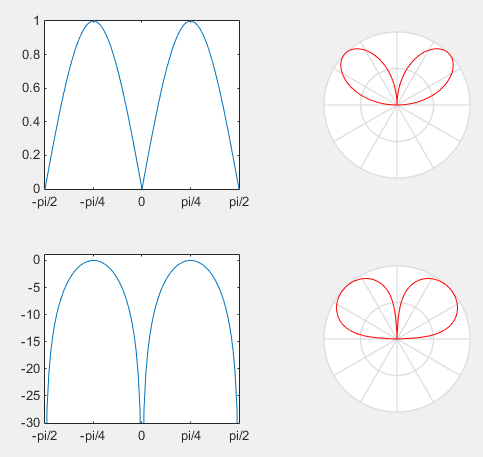
Following is the matlab code for the plot shown above. Play with this by changing theta_shift or any other values in a_theta array as you like until you get the intuitive understanding of each parameters.
theta = -0.5*pi:pi/100:0.5*pi;
d = 2.0;
theta_shift = (0.25*pi);
a_theta = [exp(-j .* 0 .* d .* (theta-theta_shift));
exp(-j .* 1 .* d .* (theta-theta_shift));
exp(-j .* 2 .* d .* (theta-theta_shift));
exp(-j .* 3 .* d .* (theta-theta_shift));
exp(-j .* 0 .* d .* (theta+theta_shift));
exp(-j .* 1 .* d .* (theta+theta_shift));
exp(-j .* 2 .* d .* (theta+theta_shift));
exp(-j .* 3 .* d .* (theta+theta_shift))];
a_theta_sum = sum(a_theta);
a_theta_sum_abs = abs(a_theta_sum);
a_theta_sum_abs = a_theta_sum_abs ./ max(a_theta_sum_abs);
a_theta_sum_abs_dB = 10 .* log(a_theta_sum_abs);
for i = 1:length(a_theta_sum_abs_dB)
if a_theta_sum_abs_dB(i) <= -30
a_theta_sum_abs_dB(i) = -30;
end;
end;
a_theta_sum_abs_dB = a_theta_sum_abs_dB - min(a_theta_sum_abs_dB);
a_theta_sum_abs_dB = a_theta_sum_abs_dB/max(a_theta_sum_abs_dB);
subplot(2,2,1);plot(theta,a_theta_sum_abs);
xlim([-pi/2 pi/2]);
set(gca,'xtick',[-pi/2 -pi/4 0 pi/4 pi/2]);
set(gca,'xticklabel',{'-pi/2' '-pi/4' '0' 'pi/4' 'pi/2'});
subplot(2,2,2);polar(theta + 0.5*pi,a_theta_sum_abs,'-r');
t = findall(gcf,'type','text');
delete(t);
subplot(2,2,3);plot(theta,10 .* log(a_theta_sum_abs));ylim([-30 1]);
xlim([-pi/2 pi/2]);
set(gca,'xtick',[-pi/2 -pi/4 0 pi/4 pi/2]);
set(gca,'xticklabel',{'-pi/2' '-pi/4' '0' 'pi/4' 'pi/2'});
subplot(2,2,4);polar(theta + 0.5*pi,a_theta_sum_abs_dB,'-r');
t = findall(gcf,'type','text');
delete(t);
Note : I posted the graphical representation of this vector in my visual note www.freetechslide.com . Check [Engineering] -> [1] -> [Radiation Pattern]. You would see the effect of parameters like 'd' in more intuitive way in the visual note.
Basic Concept : Beam Forming - Phased Array
In previous sections on basic Antenna array mode, we could see that just by arraning multiple antenna in an array we could create a beam with the directivity to a certain direction and by physically rotating the antenna array we can change the direction of the beam. However, there will be a lot of restrictions in terms of the shape of the beam and controlling the direction in simply placing multiple antenna in an array.
There are even smarter idea as invented as shown below. You can do everything explained above and do even more by placing the devices that can control phase and amplitude of a wave to each antenna as illustrated below.
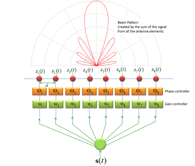
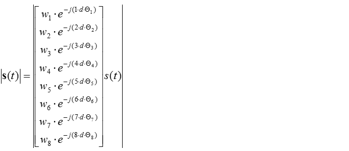
The total energy pattern (beam pattern) created by summing up all the transmitted energy coming out of each antenna can be described in mathematical form as shown below.
Again, you can simplify this long equation into a simple vector notation as shown below. Theoretically, you can create a beam with any shape and any direction by changing the gain and phase in the vector.
Note : I posted the graphical representation of this vector in my visual note www.freetechslide.com . Check [Engineering] -> [1] -> [Radiation Pattern]. You would see the effect of parameters like 'd' in more intuitive way in the visual note.
As I mentioned above, theorectically you can create a beam with any shape and any angle by chaning angle (phase) and gain connected to each antenna. Then the question is how to find proper angle (phase) and gain value to each antenna to achieve the desired beam pattern.
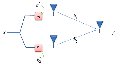
Long story.. but the conclusion is not that complicated. Let's asume that we have the simplest array antenna made up of just two antenna as shown below. The antenna array on the left is transmitter antenna and the single antenna on the right is the reciever antenna. The blocks labeled p1 and p2 is a complex number that representing phase and amplitude controller (As you know, a complex number can represent both phase and amplitude). h1 and h2 is channel coefficient between transmitter and reciever antenna.
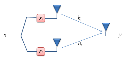
Now the question is how to represent the received signal y using these parameters. It can be presented as shown below (If you are not familiar with this kind of channel representation, refer to Channel Model page)
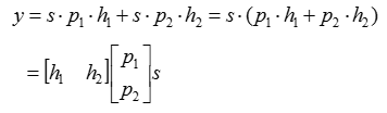
Now the question is how to find p1 and p2 value to make the beam properly point to the reciever antenna. If you rewrite the question a little bit, it can be 'what is the p1 and p2 value that maximize the received energy at the reciever antenna ?'. In real situation, h1 and h2 act as some factors distorting/deteriorating the signal between the transmitter and reciever antenna. So, if we can set p1 and p2 propery to compensate (undo) the effect of h1 and h2, that would be the p value to make the received energy maximum. h1 and h2 are complex numbers, meaning h1 and h2 has gain component and phase component. Therefore, the question becomes 'how to undo an effect caused by a complex number ?'.
Undoing a complex number is simple. Just multiplying a complex conjugate to the given complex number. (If you multiply a complex number with its conjugate, the phase of the resulting complex number become always '0', meaning that imaginary part become always 0. So in this kind of situation, we can say 'multiplying a complex number with its conjugate' is same as 'undoing the phase shift caused by the complex number'.
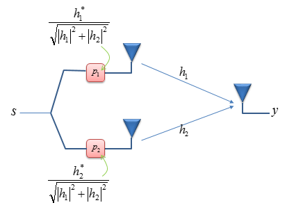
Therefore, if you put complex conjugate of h1 and h2 into p1 and p2 as shown below, this would undo the phase shifting effect of h1 and h2.
This looks very handy and simple solution. However, there is a problem with this kind of undo. By multiplying the channel coefficient with its conjudate, we can easily remove the phase part. However, the real value of the resulting number gets larger. To prevent this, you only have to normalize those conjugate numbers with the norm of h vector (a vetor made of h1 and h2) as shown below.
Now with this, we found the p1 and p2 to make the beam in the best direction to the reciever antenna.
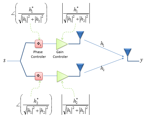
If you implement the p1 and p2 in DSP or FPGA, the illustration above is good enough. Because you can easily implement a complex number as it is. However, if we implement p1 and p2 as analog component, probably following illustration would be a better representation.
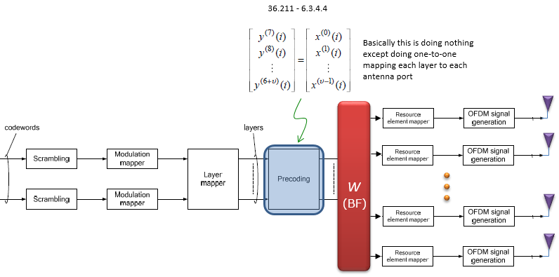
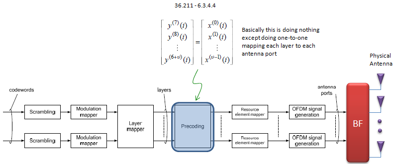
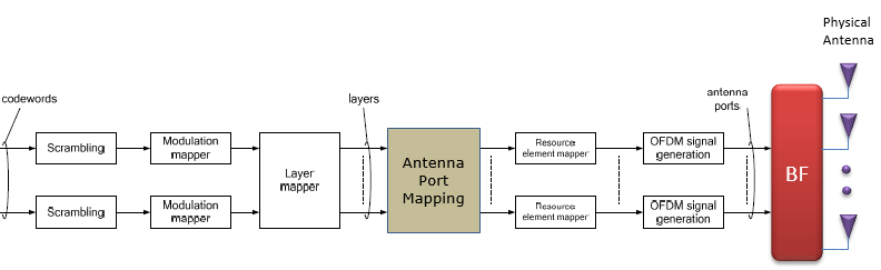
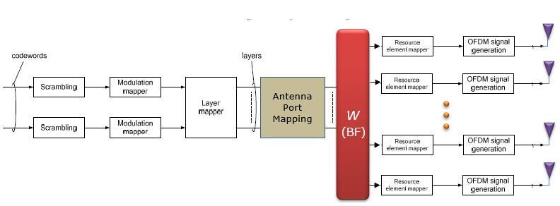
Overall procedure for LTE beamforming in the context of physical layer processing goes as shown below.
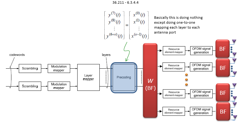
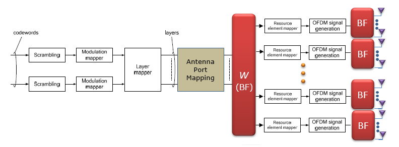
In case of BeamForming, Precoding is doing almost nothing and in stead something similar to Precoding happens at the stage labeled as BF(Beam Forming) shown below. Theoretically we can implement Beamforming in roughly three different way as illustrated below. But as far as I understand, in LTE < Case 1 > is most commonly used. (NOTE : in the system which use a lot of antenna as in 5G/NR, it is mostly likely to use < Case 3 > )
< Case 1 : Pure Baseband >
Basic Beamforming Model for this type is described in 36.101 (B.4.1, B.4.2, B.4.3) and it propose three different categories as summarized below.
< Case 2 : Pure RF >
< Case 3 : Hybrid >
< Single-layer random beamforming (Antenna port 5, 7, or 8) : 36.101 B.4.1>
This type has following two cases. TM8, DCI Format 2B single layer would fall into this type.
i) without a simultaneous transmission on the other antenna port
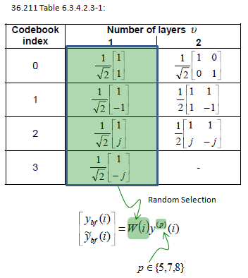
ii) with a simultaneous transmission on the other antenna port
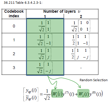
< Dual-layer random beamforming (antenna ports 7 and 8) : 36.101 B.4.2>
TM8, DCI Format 2B dual layer would fall into this type.
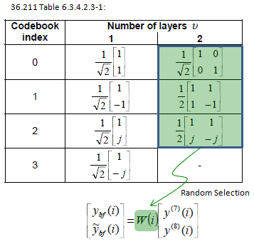
< Generic beamforming model (antenna ports 7-14) : 36.101 B.4.3 >
TM9, DCI Format 2C dual layer would fall into this type.
Unliked other model like B.4.1 and B.4.2, the definition of W(i) is not always obvious. The 36.101 B.4.3 says "The precoder matrix W(i) is specific to a test case.", it means we have to define a specific test case (situation) and then try to define the W(i).
Example 1 : 8 x 2 (8 Antenna, 2 Layers)
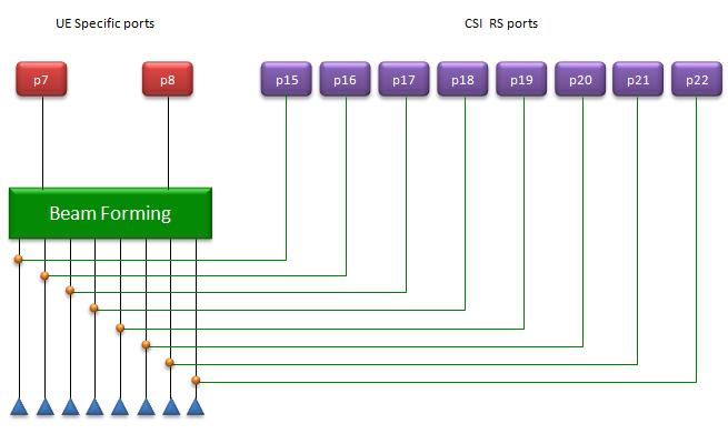
In this example, I will look into a case where two layered data is transmitted through 8 Tx antenna. Two UE specific reference signal p7, p8 are subject to BeamForming and 8 CSI RS ports (p15~p22) will be transmitted for CSI estimation on UE side. Overall mapping between antenna ports and physical antenna is as shown below.
< Mapping between Antenna port and physical antenna >
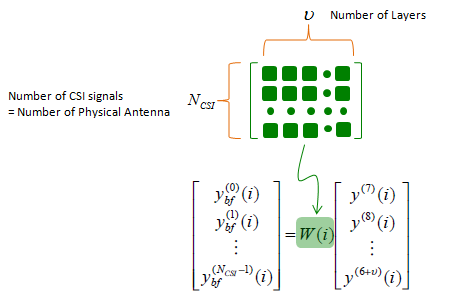
First, it seems obvious that we need something to distribute the two layered data over 8 physical antenna and it can be easily understood that we need following form of matrix.
< Beamforming Matrix converting two user ports to 8 physical antenna >
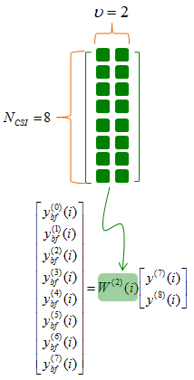
Now we have to figure out (or define) values of each matrix element. For this, we have to define our model more specifically.
36.213 7.2.4 Precoding Matrix Indicator (PMI) definition says as follows and this example is the case described by the underlined parts.
For transmission modes 4, 5 and 6, precoding feedback is used for channel dependent codebook based precoding and relies on UEs reporting precoding matrix indicator (PMI). For transmission mode 8, the UE shall report PMI if configured with PMI/RI reporting. For transmission mode 9, the UE shall report PMI if configured with PMI/RI reporting and the number of CSI-RS ports is larger than 1. A UE shall report PMI based on the feedback modes described in 7.2.1 and 7.2.2. For other transmission modes, PMI reporting is not supported
The exact value of the matrix is determined by UE PMI report and network construct the matrix W(i) based on following table.
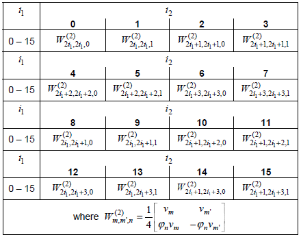
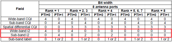
36.213 Table 7.2.4-2 Codebook for 2-layer CSI reporting using antenna ports 15 to 22
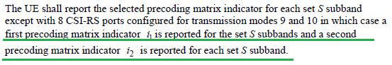
The first thing that confuses me was "Where is i_1 and i_2 is defined ?" and what do they mean (indicate) ? These are described in 36.213 section 7.2.1 "Wideband feedback -> Mode 1-2 description" as shown below. Of course it will take a long time to understand real meaning of these variable. (First you have to understand everything on CQI/RI Feedback type page first just to understand these i_1 and i_2)
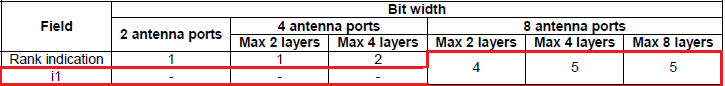
Following is more detailed information from 36.212 regarding the i1 and i2 report from UE.
< 36.212 - Table 5.2.3.3.1-3A: UCI fields for joint report of RI and i1 (transmission mode 9 configured with PMI/RI reporting with 2/4/8 antenna ports and transmission mode 10 configured with PMI/RI reporting with 2/4/8 antenna ports) >
< 36.212 - Table 5.2.3.3.2-2B: UCI fields for channel quality feedback for UE-selected sub-band reports (transmission mode 9 configured with PMI/RI reporting with 8 antenna ports and transmission mode 10 configured with PMI/RI reporting with 8 antenna ports) >
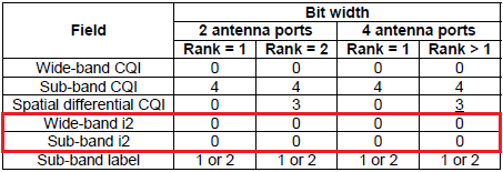
< 36.212 - Table 5.2.3.3.2-2B: UCI fields for channel quality feedback for UE-selected sub-band reports (transmission mode 9 configured with PMI/RI reporting with 8 antenna ports and transmission mode 10 configured with PMI/RI reporting with 8 antenna ports) >
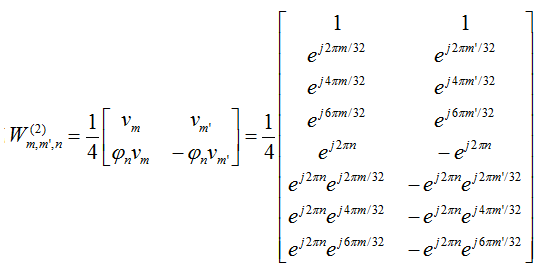
Now let's look into more details of W(i) matrix. Let's construct the generic form of W(i) matrix for this case. The matrix is defined at the bottom of the table shown above.
You would notice that W(i) is made up of following two components.
With Reference to 36.213 7.2.4
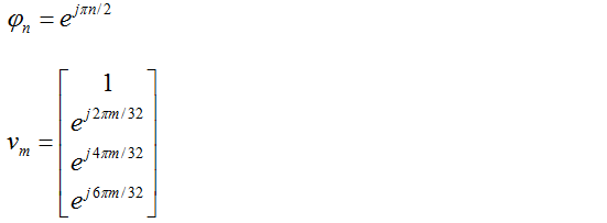
With the two components, you can contruct the generic form of W(i) matrix as shown below. For each specific case, we have to figure out n,m',n to fill out the matrix with specific values. and n,m',n is determined by the PMI report and Table 7.2.4-2.
With Reference to 36.213 Table 7.2.4-2
As described above, the key issue of Beamforming implementation is how to figure out proper BeamForming matrix for each transmission. As in a common MIMO technology, we can think of roughly a couple different approach as below.
i) Open Loop Method : This is based on the assumption that a Network 'SOMEHOW' knows the proper beamforming matrix without any information from UE. Ideally we can think of two approaches as below. (Practically the method a) would not be of much meaning)
a) Applying the same Beamforming matrix for all the transmission
b) Applying the dynamically chaning Beamforming matrix but not based on specific UE Report
ii) Close Loop Method : This is the method where a Network generate the proper beamforming matrix based on specific report from UE. For this purpose, network transmit a specific pilot signal called (CSI-RS) and UE evaluate the it's receiving signal quality based on the received CSI-RS and report the result to Network. (For the CSI-RS configuration being used in LTE for this purpose, refer to CSI-RS and Periodicity section)
Beamforming in 5G/NR (Massive MIMO)
In NR specification, one of the most outstanding difference you may notice in terms of physical layer processing would be that there is no Precoding stage in downlink process(See the PDSCH transport and physical layer processing page). However, you still see the precoding process in Uplink process(See the PUSCH transport and physical layer processing page).
I think the main reason of excluding Precoding in downlink process would be that it is for certain that we need to use Massive MIMO especially in mmWave spectrum. but there are some fundamental questions to be answered in NR MassiveMIMO/BeamForming. Would 3GPP specify any details on how to implement the MassiveMIMO/Beamforming ? or just leave everything to gNB manufacturer ? Are they going to apply Massive MIMO/Beamforming in sub 6 Ghz range as well ? If they decided not to use it, how to handle the possible problems caused by missing Precoding step ? These are some of the questions in my mind for now.
You may noticed that I used the term MassiveMIMO and BeamForming as almost the same meaning, but technically MassiveMIMO is not necessarily same as BeamForming. The term 'Beam Forming' is pretty clearn concept as described above, but the term MIMO(Multiple Input Multiple Output) is getting more and more blurry concept. It seems that people tend to call a system a MIMO almost automatically if they see any system using multiple Tx antenna and multiple Rx antenna. This kind of simple interpretation would not be a big problem until LTE (at least in TM3, TM4), but in 5G 'Multiple Tx/Rx antenna = MIMO' rule may not always be true.
When we say 'MIMO', it usually mean it as a mean to transfer multiple streams of data simultaneously to increase data throughput. More accurately this should be called as 'Spatial Multiplexing'. To do this, we use multiple Tx antenna and multiple Rx antenna. However, when we say 'Massive MIMO' in 5G, it does not necessarily imply the way of increasing throughput, the major purpose of what we call 'Massive MIMO' is to implement Beam Forming (I personally think the term 'Massive MIMO' is a little misleading term). I would suggest you to refer to following notes for Massive MIMO
Regarding the implementation of NR/5G Beamforming/MassiveMIMO, overall guide lines and rrc configuration for beam management is defined in the specification as described in BeamManagement and CSI Codebook. But the detailed implementation of Hardware is still left up to the implementation by infrastructure vendors.
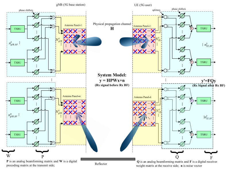
In NR, especially for FR2 where a huge number of antenna is used, it would use hybrid (or Pure RF type) of implementation due to the reason mentioned in this paper ([4]) as quoted below.
When antenna scale is so large, fully exploiting multiple-input multipleoutput (MIMO) gain by pure digital beam-forming in baseband is not realistic due to the problems on hardware cost, power consumption and standardization complexity since it requires dedicated RF chain for each baseband antenna port. Therefore, multi-antenna schemes considering hybrid analog-digital beam-forming is supported in NR to reduce the cost and complexity of 5G equipment.
< Case 1 : Pure RF >
< Case 2 : Pure Baseband >
< Case 3 : Hybrid >
A more detailed illustration of Hybrid Beamforming presented in this paper ([4]) is shown below. (NOTE : In real implementation, UE side antenna is not as complicated as below. In general, UE is using a few modules (panel) of antenna which is made up of several (usually 4) antenna elements. For Antenna and Beamforming on UE side, refer to this note)
YouTube :
Following videos are mostly about the general concept and application of beam forming and they are not specifically limited to LTE beamforming.
NOTE : The wireless technology most commonly and widely adopting the beamforming would be 5G/NR. For those videos with 5G application, refer to this list.
-
BeamForming (Feb 2011)
-
802.11ac: Why Beamforming? (May 2013)
- Antenna parameters (Feb 2013)
- Various forms of Antenna array (Feb 2013)
- Antenna array part-I (May 2013)
- Addressing LTE-A Beamforming Test Challenges: Part 1. Measurement Challenges (Oct 2016)
- Addressing LTE-A Beamforming Test Challenges: Part 2. Key Measurements (Oct 2016)
- Addressing LTE-A Beamforming Test Challenges: Part 3. Using a Multi-Channel Reference Solution (Oct 2016)
- Full-Stack Hybrid Beamforming in mmWave 5G Networks (Jun 2021)
References :
These are not my posting, but I would like to recommend these for further understanding and giving you different perspective.
[2] TD-LTE 8-antenna dual-stream beamforming technology
[3] Advanced antenna systems for 5G networks
[4] Beam Management in Millimeter-Wave Communications for 5G and Beyond
YouTube :
- Build Your Own Phased Array Beamformer - Jon Kraft (2022)
- Monopulse Tracking with a Low Cost Pluto SDR - Jon Kraft (2022)
- Implementing Time Delay For a Low Cost Digital Beamformer - Jon Kraft (2022)
- Rapid Phased Array prototyping with Analog Devices and X-Microwave - Jon Kraft (2022)