|
Engineering Math - Differential Equation |
||
|
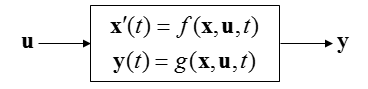
State Space Modeling
When you are given with relatively simple differential equations, you would normally solve those equation in computer using a regular DE solving function (like ode functions in Matlab or DSolve, NDSolve in Mathematic etc). However, if you save very complicated set of differential equations or multiple equations linked together to represent a system, many engineers turn to various System Simulation tools (like Matlab Simulink) using various block diagram. Usually those tools provide various additional blocks (function) which is hard to be included in the regular DE solvers mentioned above. You would find it very powerful and apealing once you saw a lot of fancy examples provided those system simulation tools. However, if you are asked to solve a problem using those system simulation tool you may be quite embarrased and you might ask yourself 'I have all the equations representing each components in my system, but how can I convert these equations into the diagrams that is required for the tools ?'. And you may find it not easy to learn those tricks. If you haven't learned about the technics seriously, it would be difficult to make sense out of what somebody else has done, not to mention to drawing those diagram by yourself. In this page, I will try to show you how to convert various equations to those System Diagram (or Simulation Diagram) using various examples. Unfortunately I don't think there is clear and simple rules to convert the equations to diagram. In most cases, you would need to rely on various thumb rules. Only a lot of practice would give you good understandings on it.
Some of the rules I would suggest you to keep in mind are a) Once you are given an equation, separate the terms of highest order differntial terms from the remaining terms. In my case, I usually rearrange the equation so that the hightest terms are at the left hand side and the remaining terms on the right hand side of the equation. b) Once you have done the rearrangement, modify the equation so that the coefficient of the highest order term is '1'. c) Once you are done with above steps, identify which variable (or terms) is acting as input and which one is acting as output (I would suggest you to draw a rectangle around the equation and put the input arrow(s) on the left side and output arrow(s) on the right side.) Most of the examples shown in this page is based on the assumption that you are already applied the rule a) and b). (In some examples, I would start from an equation that hasn't done this just for practice).
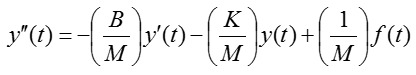
In this example, you are given an equation as follows. As you see, this is given already done with rule a) and b), meaning you can use this equation as it is without any rearrangement.
Now let's do rule c). i.e, let's identify the input and output in the equation. How do we identify them ? Actually just by looking at the equation, it would be hard to identify them. You should look into the physical system itself from which the given equation is driven. However, since derivation of the equation from the physical system is not the scope of this page, I will just give you the input and output as shown below.
From the equation, I think you can draw a diagram as shown below and I don't think you need any further explanation about this.
Is the above diagram complete ? No. Why not ? The biggest reason is that there is not output coming 'OUT OF' the system. Then let's put down an arrow indicating the output as follows. As you see below, adding an output arrow is easy, but think of how to connect the output arrow to the existing diagram.
With what you have learned in Differential Equation class, you may connect the two separate parts by adding integration blocks as shown below.
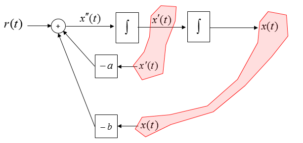
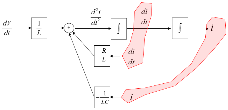
Now you see some of the same variables showing up at different places as highlighted below.
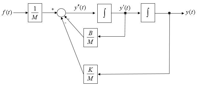
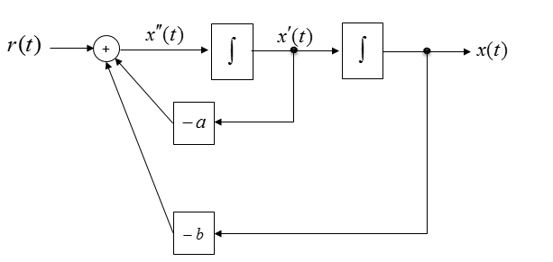
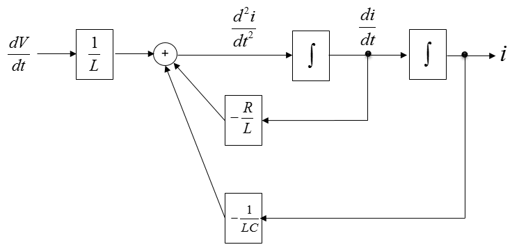
Connect each of these same variables with arrows and then you will get a complete system diagram (simulation diagram) as shown below.
In some system diagram (or simulation tool), you may need to represent things in laplace notation. Then you can represent the above diagram using laplace notation as shown below.
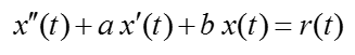
Now you are given another equation as shown below.
As you see, in this equation the highest order deferential term is not isolated. So you would need to apply the rule (a) first, meaning that you need to rearrange the equation in such a way that the highest deferential term is separated from other terms as shown below.
Since the coefficient of the highest order term is 1, you don't need to apply rule b).
Now let's do rule c). i.e, let's identify the input and output in the equation. How do we identify them ? Actually just by looking at the equation, it would be hard to identify them. You should look into the physical system itself from which the given equation is driven. However, since derivation of the equation from the physical system is not the scope of this page, I will just give you the input and output as shown below.
From the equation, I think you can draw a diagram as shown below and I don't think you need any further explanation about this.
Is the above diagram complete ? No. Why not ? The biggest reason is that there is not output coming 'OUT OF' the system. Then let's put down an arrow indicating the output as follows. As you see below, adding an output arrow is easy, but think of how to connect the output arrow to the existing diagram.
With what you have learned in Differential Equation class, you may connect the two separate parts by adding integration blocks as shown below.
Now you see some of the same variables showing up at different places as highlighted below.
Connect each of these same variables with arrows and then you will get a complete system diagram (simulation diagram) as shown below.
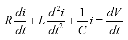
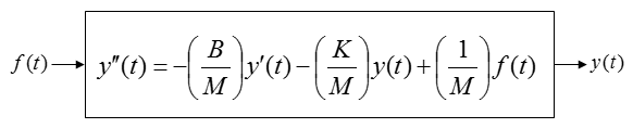
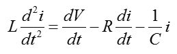
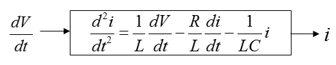
Now you are given an equation as follows. This is the form you should apply rule a), b), c) all together.
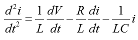
Applying the rule a), you can rearrange the equation as shown below.
Applying the rule b), you can rearrange the equation as shown below.
Now let's do rule c). i.e, let's identify the input and output in the equation. How do we identify them ? Actually just by looking at the equation, it would be hard to identify them. You should look into the physical system itself from which the given equation is driven. However, since derivation of the equation from the physical system is not the scope of this page, I will just give you the input and output as shown below.
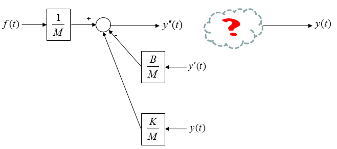
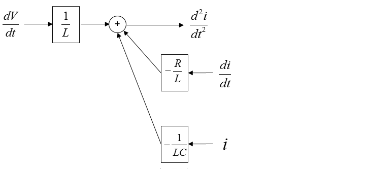
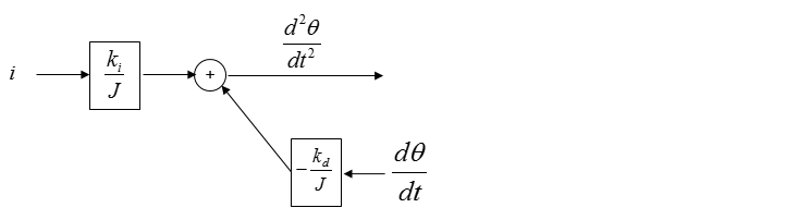
From the equation, I think you can draw a diagram as shown below and I don't think you need any further explanation about this.
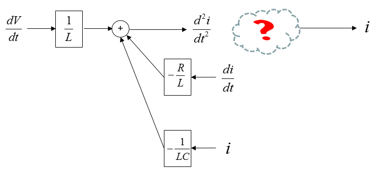
Is the above diagram complete ? No. Why not ? The biggest reason is that there is not output coming 'OUT OF' the system. Then let's put down an arrow indicating the output as follows. As you see below, adding an output arrow is easy, but think of how to connect the output arrow to the existing diagram.
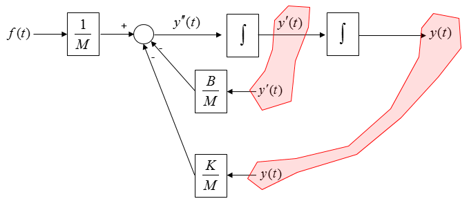
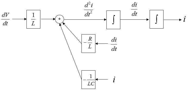
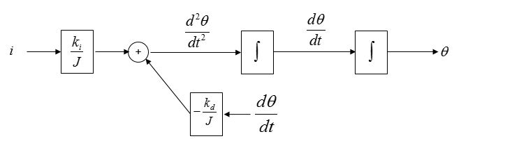
With what you have learned in Differential Equation class, you may connect the two separate parts by adding integration blocks as shown below.
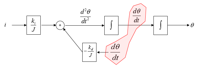
Now you see some of the same variables showing up at different places as highlighted below.
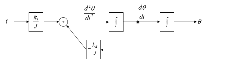
Connect each of these same variables with arrows and then you will get a complete system diagram (simulation diagram) as shown below.
Now we are give a little bit more complicated equation, a system equation that are made up of two equations as shown below.
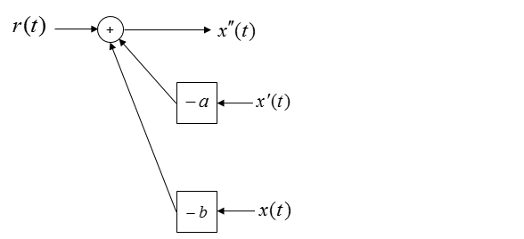
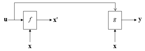
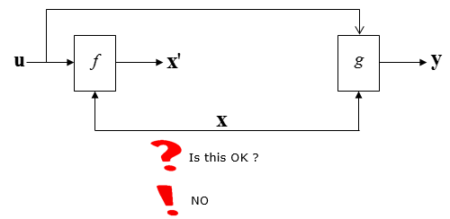
Just by looking at the equation, you would be able to draw a following diagram and you wouldn't need any further explanation about this.
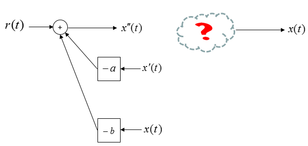
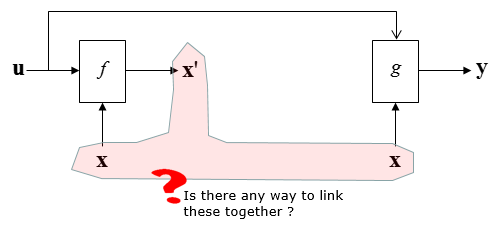
Now you would have question as shown below.
The first thing you may try is to connect the same variable x as shown below. But this is not correct since a connection line is not allowed to have the arrow head on both sides.
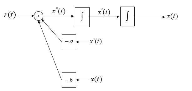
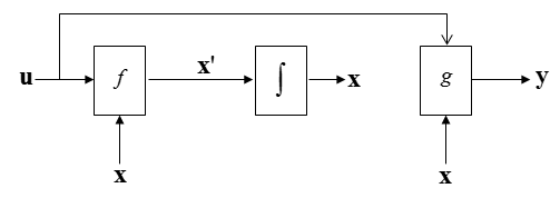
Then, let's add a integration block to x' and you would have following diagram.
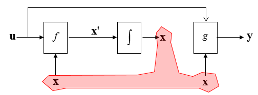
Now you see three same variable that are not connected.
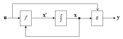
Let's connect these three variables with arrows as shown below. Now all the variable x are connected by arrows with single head as shown below.
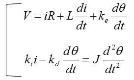
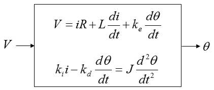
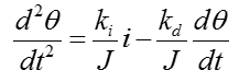
Now we are give a simultaneous differential equation (a set of equation) as shown below. This is the system equation derived from a DC motor. If you want to know how this is derived, refer to DC Motor in Electro mechanics page.
Let's identify the input and output in the equation. How do we identify them ? Actually just by looking at the equation, it would be hard to identify them. You should look into the physical system itself from which the given equation is driven. However, since derivation of the equation from the physical system is not the scope of this page, I will just give you the input and output as shown below.
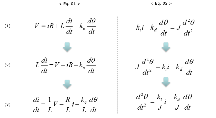
Now let's apply the rule (a), (b) and you will get the two equations as shown below.
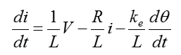
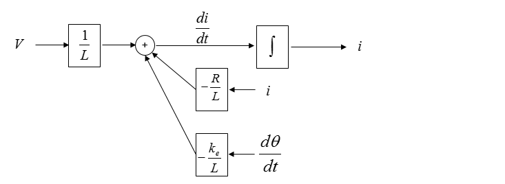
Let's start with the drawing the simulation diagram for the first equation < Eq. 01 >
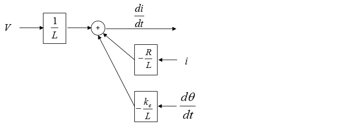
You can draw the first step diagram as shown below without thinking much.
Do you think the diagram shown above is good enough ? Of course No. How can we improve this ? In case of the single equation diagram, we usually improved the first step diagram by adding the output of the system (See single equaion examples shown above). However, in case of multi equation system it would be a little bit tricky to improve the first level diagram because the output of each equation may not be obvious some times. Try some of your intuition you have build from previous single equation examples. I just added an integration block as shown below.
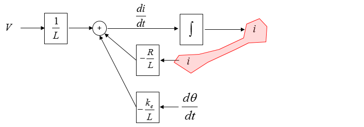
Once you extended this way, now you see a common parameter as shown below.
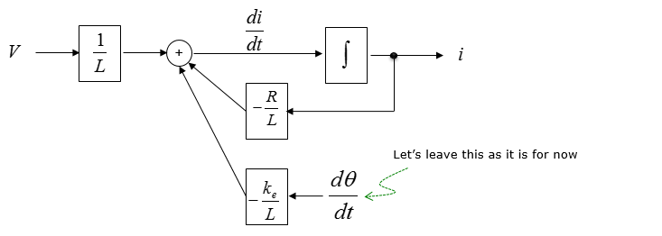
Now you can connect the same parameter with a line as shown below
You still have a dangling parameter to be connected somewhere else. However, there is no way to improve it in this diagram as of now. So let's leave it as it is until we complete the diagram for the second equation.
Now let's take a look at the second equation and draw the simulation diagram for it.
You can draw the first step diagram as shown below without thinking much.
Do you think the diagram shown above is good enough ? Of course No. How can we improve this ? In case of the single equation diagram, we usually improved the first step diagram by adding the output of the system (See single equaion examples shown above). However, in case of multi equation system it would be a little bit tricky to improve the first level diagram because the output of each equation may not be obvious some times. Try some of your intuition you have build from previous single equation examples. I just added an integration block as shown below.
Once you extended this way, now you see a common parameter as shown below.
Now you can connect the same parameter with a line as shown below
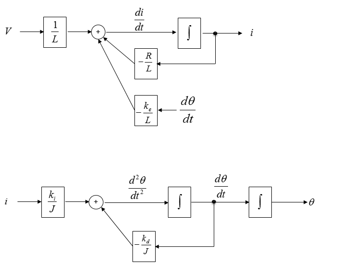
Now we have two separate diagram for the two separate equations. Now let's put these two diagram on a same sheet of paper as shown below.
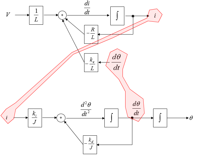
Now let's see if there are any common variables across the two diagram. I see the common variables as marked below.
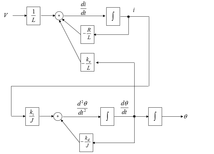
Connecting the common variables with arrows, we will get a combined diagram as shown below. This is the final diagram for the simultaneous equation.
Reference :
[1] Simulation - Block Diagram Notation [2] DC Motor Position: Simulink Modeling [3] Suspension: Simulink Modeling [4] Cruise Control: Simulink Modeling [5] Spectrum : Solving Differential Equation
|
||