As you may guess from the word itself, deconvolution is 'de' - 'convolution', meaning 'undo convolution'. As I mentioned in Overview page, the transmitted signal always get distorted as it go through a channel and the reciever gets the distorted signal. The mechanism of the distortion can be modeled by a mathematical technique called 'Convolution'. If the degree of the distortion is not so serious, we don't have to worry about it and with just a little bit of additional care for reciever design, we can decode signal without any error. But in reality the level of distortion tend to be greater than we hope.

Then what we can do to decode the received signal (distorted signal) properly ? One possible solution would be as shown below.

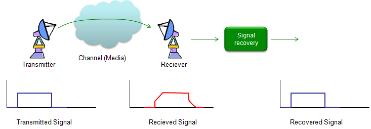
• The upper row is the physical path. A transmitter sends, the signal crosses the Channel (Media) cloud, and a receiver picks it up.
• The lower row shows the same three points as waveforms. The Transmitted Signal is a clean rectangular pulse, the Recieved Signal is the red rounded and sloped version of it, and the Recovered Signal is rectangular again.
• The Signal recovery box sits after the receiver, so it works on what arrived rather than on what was sent.

• Example 1 : a decaying exponential channel
• Example 2 : an oscillating channel
• Why deconvolution is not the whole answer
• When the channel is not known : blind deconvolution

Let's assume that we have the distorted signal as shown above (red line) and the level of distortion is too serious. If we can design a special 'Signal recovery' box that can recover the original signal (undistorted signal) from the distorted signal, it would solve our problem. One of this 'Signal Recovery' technique is 'Deconvolution'. As you see the illustration below, the distorted signal is created by the convolution of the transmitted signal and channel impulse response. The original signal (undistorted signal) can be recovered by the deconvolution of the recieved signal and channel impulse response.

There is a very important thing that you have to notice. As you see in the illustration, we have to know the impulse response (charateristic information) of the channel in order to recover the signal by deconvolution. So characterizing a channel (estimating a channel) is also very important part of communication technology. If the channel characteristic does not change (static), we can get the characteristics in those methods explained in impulse response section, but if the channel characteristics changes dynamically we need another special technique called 'channel estimation'. (I will cover on this later in a separate section).

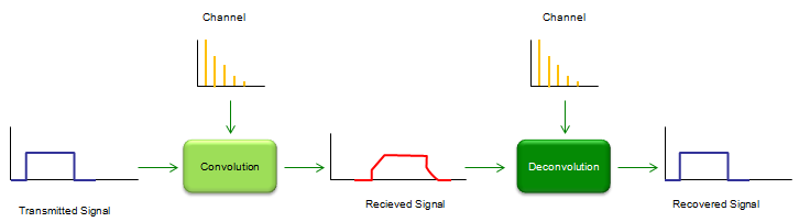
• The same chain is redrawn with the operations named. Convolution turns the Transmitted Signal into the Recieved Signal, and Deconvolution turns it back.
• Both boxes take a second input from above, and in both cases that input is the Channel, drawn as the same decaying impulse response.
• The two boxes therefore depend on the same information. An error in the channel estimate enters the recovery as directly as it entered the distortion.

Example 1 : a decaying exponential channel

Here goes a couple of examples for deconvolution. Basically it is about the same channel that I used in convolution example. Starting with the distorted signal first and deconvolute the distorted signal with the same channel and get the recovered signal. Just playing with this code would be better than my explanation.

 

x = [0 1 0 1 0 1];

 

sf = 20; % samples per bit

p_x = x;

 

if sf > 1

   for i = 2:sf

    p_x= [p_x ; x];

   end

 

   p_x = reshape(p_x,[],1);

end

 

a = 0.5;

t = 0:10;

k = 0.3;

chan = 0.5*exp(-k*t); % this is to create the characteristic response (impulse response) of a channel

chan = chan/sum(chan);

 

w = conv(p_x,chan); % this create the distorted signal by convoluting the original signal and the channel

y = deconv(w,chan); % this recovers the original signal by decovoluting the distorted signal and the channel

 

subplot(2,5,[1 2]);stem(w);axis([1 length(w) -1.5 1.5]);title("rx signal");

subplot(2,5,3);stem(chan,'MarkerFaceColor',[0 0 1]);axis([1 length(chan) -0.5 0.5]);title("chan");

subplot(2,5,[4 5]);stem(y);axis([1 length(y) -1.5 1.5]);title("deconvoluted signal");

subplot(2,5,[6 7]);plot(w);axis([1 length(w) -1.5 1.5]);title("rx signal");

subplot(2,5,8);stem(chan,'MarkerFaceColor',[0 0 1]);axis([1 length(chan) -0.5 0.5]);title("chan");

subplot(2,5,[9 10]);plot(y);axis([1 length(y) -1.5 1.5]);title("deconvoluted signal");

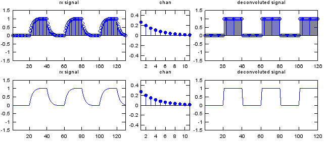
• The left panel is titled rx signal and holds w, the convolution of the input with the channel. The rectangular pulses have lost their edges and sag between transitions.
• The middle panel is titled chan and shows the impulse response, a decaying exponential normalised so that its samples sum to 1.
• The right panel is titled deconvoluted signal and holds y. The rectangular pulses are back, with square edges and flat tops.

The normalisation line matters more than it looks. Dividing chan by its own sum makes the channel pass the signal without changing its level, so the recovered pulses return at the height of the originals rather than scaled.

The recovery is exact here because nothing was lost. The code convolves and then deconvolves the same array with the same channel, and no noise is added anywhere, so deconv can undo what conv did sample for sample.

Example 2 : an oscillating channel

The channel changes from a decaying exponential to a decaying oscillation, so its taps alternate in sign instead of all being positive. The distortion that produces looks quite different from the one above, and the recovery still works.

x = [0 1 0 1 0 1];

sf = 20; % samples per bit

 

p_x = x;

if sf > 1

   for i = 2:sf

    p_x= [p_x ; x];

   end

 

   p_x = reshape(p_x,[],1);

end

 

a = 0.5;

t = 0:10;

k = 0.3;

chan = 0.5*exp(-k*t).*cos(pi*t);

chan = chan;

chan = chan/chan(1);

 

w = conv(p_x,chan);

y = deconv(w,chan);

 

subplot(2,5,[1 2]);stem(w);axis([1 length(w) -1.5 1.5]);title("tx signal");

subplot(2,5,3);stem(chan,'MarkerFaceColor',[0 0 1]);axis([1 length(chan) -1.5 1.5]);title("chan");

subplot(2,5,[4 5]);stem(y);axis([1 length(y) -1.5 1.5]);title("rx signal");

subplot(2,5,[6 7]);plot(w);axis([1 length(w) -1.5 1.5]);title("tx signal");

subplot(2,5,8);stem(chan,'MarkerFaceColor',[0 0 1]);axis([1 length(chan) -1.5 1.5]);title("chan");

subplot(2,5,[9 10]);plot(y);axis([1 length(y) -1.5 1.5]);title("rx signal");

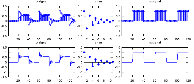
• The middle panel is titled chan and shows the oscillating impulse response. It starts at 1 and alternates in sign, so successive taps pull the signal in opposite directions.
• The panel titled tx signal holds w, the distorted waveform. The pulses now ring rather than sag, with overshoot at each edge.
• The panel titled rx signal holds y, the recovered signal, and its rectangular pulses are clean again.

Two titles in the figure above do not match what the panels hold. The distorted waveform is labelled tx signal when it is the channel output, and the recovered waveform is labelled rx signal when it is the deconvolution output. Example 1 labels the same two panels rx signal and deconvoluted signal, which is the right way round.

One line of the code above has been corrected as well. It read y = deconv(p_w,w), and p_w is defined nowhere on the page, so the line could not run. The call that matches both the figure and Example 1 is y = deconv(w,chan).

Why deconvolution is not the whole answer

Both examples recover the input exactly, and that result is worth distrusting. Nothing in either run carries noise, and a real receiver never has that luxury. Adding noise changes the outcome completely.

Deconvolution divides. Convolution in the time domain is multiplication in the frequency domain, so undoing it means dividing by the frequency response of the channel. Wherever that response is small, the division is by a small number, and any noise sitting at that frequency is multiplied up along with the signal.

The exponential channel of Example 1 makes the point. A decaying exponential is a low pass response, so its high frequency content is weak, and dividing by it amplifies exactly the part of the spectrum where the signal is weakest. With no noise present the division is harmless. With noise present it becomes the dominant error.

Receivers therefore rarely deconvolve outright. They use an equalizer instead, which is deconvolution with a limit on how far the division may go. Zero Forcing inverts the channel completely and accepts the noise amplification that follows. MMSE holds the inversion back wherever the noise would dominate.

The other requirement is the one the introduction already names. Both equalizers need the channel, and so does plain deconvolution, so none of this runs before channel estimation has produced an estimate. An error in that estimate enters the recovery directly.

When the channel is not known : blind deconvolution

The section above assumes that a channel estimate exists. Sometimes none does. A recording may arrive with no pilot in it, or the distortion may have been applied long before anyone thought to measure it. Recovering the signal without knowing the channel is called blind deconvolution, and it is harder than it first appears.

Why the problem has no unique answer

Start from the polynomial form. Convolution in time is multiplication of polynomials in z^-1, so the received sequence satisfies Y(z) = H(z) X(z). The roots of Y are then the roots of H and the roots of X, gathered into a single set.

That is the whole difficulty in one line. Recovering the channel means deciding which of those roots belonged to it. Any subset of the right size gives a valid factorisation, and every one of them reproduces the received data exactly. For the wrong choices the residual is not merely small. It is zero.

Counting samples makes the same point more gently. An input of N samples and a channel of M samples produce N + M - 1 received samples, against N + M unknowns. The data falls one short before noise is considered at all.

An extra assumption is therefore not a refinement here. It is what creates a unique answer, and every method below is named by the assumption it makes.

The shape that every method shares

Blind methods look different on the page and are largely the same underneath. Each one minimises the same cost, with a different penalty attached to the input, to the channel, or to both of them.

The cost is the squared error between the received data and h convolved with x, plus those two penalties. Two unknowns appear multiplied together, so the cost is not convex in the pair. The usual way round that is to alternate.

• Hold h fixed and solve for x. That is exactly the regularised problem of the section above, and it is linear.
• Hold x fixed and solve for h. The same linear problem, with the two roles exchanged.
• Rescale so the channel keeps unit energy, then repeat until the estimates stop moving.

Three failures catch everyone who writes this loop for the first time.

• The starting point decides the answer. The cost is not convex, so the loop settles into whichever factorisation it began near.
• A one sample channel fits perfectly. Setting h to a single impulse and x to the received data drives the squared error to zero, so a penalty has to rule that out.
• The scale drifts. Multiplying h by a constant and dividing x by the same constant leaves the cost unchanged, so one of the two must be pinned every pass.

The second failure is worse than it sounds. Estimating both unknowns together favours the no distortion answer rather than merely tolerating it. The stronger methods therefore estimate the channel with the input averaged out, rather than solving for the two side by side.

Constant modulus algorithm

This method never estimates the channel at all. It adapts the recovery filter directly, and it works whenever the transmitted symbols all carry the same amplitude. QPSK satisfies that exactly, which is why the algorithm is the most widely deployed blind method in digital radio.

The filter is adjusted to drive the output amplitude towards a constant. The cost is the squared difference between the squared output magnitude and a target value, averaged over symbols, and a stochastic gradient step minimises it. Nothing in the loop needs to know which symbols were sent.

Two properties matter in practice. The cost carries local minima, so a poor start can settle on the wrong filter. The output also arrives rotated by an unknown phase and delayed by an unknown number of symbols, which is the ambiguity of the first sub-section returning in a smaller form. Differential encoding or a single pilot resolves it.

Cyclostationary and subspace methods

Second order statistics alone cannot identify a channel from a stationary input. The autocorrelation of the received signal carries the magnitude of the frequency response and discards its phase, so two channels differing only in phase look identical. That result rules out the cheapest approach.

Sampling faster than the symbol rate changes the situation. One channel sampled at twice the symbol rate behaves as two channels driven by the same input, and the cross correlation between the two carries the phase that each one alone had lost. The channel then follows from second order statistics after all.

The condition is that the two sub-channels share no common root. Where they do, the shared factor stays invisible and the estimate fails. That is the root partition problem of the first sub-section, reappearing as a concrete requirement on the sampling.

Higher order statistics

A different way past the phase problem is to stop using second order statistics. Moments beyond the second retain phase information, provided the transmitted symbols are independent and not Gaussian. Fourth order cumulants are the usual choice.

The price is data. Cumulant estimates converge far more slowly than correlation estimates, so these methods need long records before the channel estimate becomes usable. They are close relatives of independent component analysis, which solves the same separation problem from the same assumption.

Cepstral separation

The cheapest method that ever works begins with a logarithm. Taking the log of the spectrum turns the product of channel and input into a sum, and the inverse transform of that log spectrum is called the cepstrum. A sum is far easier to split than a product.

Separation then needs the two parts to occupy different regions of the cepstrum. A short smooth channel lands near the origin and a long spiky input lands further out, so a simple window keeps one and discards the other. Speech analysis separates the vocal tract from the excitation in exactly this way.

It fails when the two regions overlap, and unwrapping the phase of the log spectrum is a persistent nuisance in any implementation.

Minimum entropy and sparse methods

Seismic work makes the opposite assumption to the constant modulus algorithm. The input there is a reflectivity sequence, mostly zero with occasional large spikes, so the recovery filter is chosen to make its output as spiky as possible rather than as flat as possible.

Kurtosis is the usual measure of spikiness, and maximising it over the filter coefficients is the whole algorithm. The modern form replaces kurtosis with an L₁ penalty on the input inside the alternating loop above, which behaves better and combines more easily with other constraints.

Which one to reach for

The choice follows from what is known about the transmitted signal, rather than from anything about the channel. The table below maps each method to the assumption that makes it work, and that assumption is the thing to check first.

One entry is missing from that table on purpose. No row covers a 3GPP receiver, because the standards are written so the blind problem never arises. A pilot is inserted, the channel is measured from it, and the recovery runs with the channel known.

That is worth reading as a design decision rather than an omission. Pilots cost overhead on every transmission, and the standards pay that cost to avoid an ill posed problem entirely. Blind methods survive where a pilot cannot be inserted, or where the overhead would cost more than the difficulty of going blind.