Frris' Transmission Equation is an equation that shows the relationship between the received power and various factors influencing the received power. It is the starting point of every link budget, because it gives the received power in the simplest case: two antennas in free space.

Let's use the equation to answer three questions in turn. What does the equation describe, how does the received power depend on each factor, and how far can a link reach? The last question is where the title of this page comes from, and it is also where the free space assumption matters most.

• What does the Friis equation describe ?
• How does the received power depend on each factor ?
• How far can a link reach ?

What does the Friis equation describe ?

The equation describes one simple link: a transmitter and a receiver in free space, with nothing in between. That assumption is its strength and its limit. It gives the best case that any real link can reach, so it is the baseline for every link budget.

To get a clearer understanding, let's think of a communication system that is made up of one transmitter RF front end and one reciever front end as illustrated below.

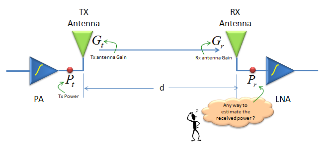
One transmitter, one receiver and the distance d between them. Pt and Pr are measured at the antenna ports, so the PA and the LNA stay outside the equation.

• Left side shows Transmission RF Front End. Gt represents the gain of the transmission antenna, PA represents a power amplifier and Pt is the power measured right before the transmission antenna.
• Right side shows Reciever RF Front End. Gr represents the gain of the reciever antenna, LNA represents a low noise amplifier and Pr is the power measured right after the reciever antenna.
• d stands for the distance between the transmitter and reciever antenna.
• lamda (not shown in the illustration) stands for wave length of the signal. As you know, lamda can be expression as c/f (speed of light / frequency).

Note where Pt and Pr sit in the drawing. Pt is the power at the input of the transmit antenna, after the PA and any cable. Pr is the power at the output of the receive antenna, before the LNA. So the equation describes only the two antennas and the space between them. Cable loss, PA output power and LNA noise figure are added separately in a link budget.

The equation also has two conditions. The first is free space: no ground reflection, no obstacle and no multipath. The second is the far field of both antennas. For an antenna of largest size D, the far field is usually taken to start at a distance of 2D²/λ. Closer than that, the antenna gain is not yet a fixed number, and the equation does not hold.

• The equation describes the space between two antenna ports : PA, LNA and cable losses are outside it.
• It assumes free space : there is no reflection, no obstacle and no multipath.
• It holds only in the far field : beyond about 2D²/λ from each antenna.

How does the received power depend on each factor ?

The equation has only five inputs, and each one moves the received power in a simple way. The dB form shows that most clearly, because every factor becomes a term that is added or subtracted.

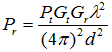
With all of these variables (factors), the received power (Pr) can be estimated by the equation shown below. This is Frris' Transmission Equation.

Following is the equation expressed in dB scale and that's why all the power and Gain parameters are combined by '+' or '-'.  You don't have to memorize this equation, just try to understand some basic charicteristics. Just looking at the equation, you would notice

• Recieved Power is proportional to Transmission Power (Very Intuitive)
• Recieved Power is proportional to Transmission Antenna Gain (Intuitive)
• Recieved Power is proportional to Reciever Antenna Gain (Intuitive).
• Recieved Power is proportional to Wave length of the signal (more accurately wavelength squared). It means Recieved Power is Anti-proportional to frequency. As frequency goes higher, received power goes lower when the same power of signal is transmitted.
• Recieved Power is inversely proportional to distance (more accurately distance squared)(Intuitive)

If you represent the same equation in linear scale, it can be represented as follows. As I said, the equation shown above is in dB scale meaning 'Log' scale. If you convert the Log scale into linear scale with high school math, you should get the following equation.

By rearranging this equation, you can represent the same equation in many different forms as shown below. You would see many different form of this equation on various different document. It would take some time until you realize all those seeminly different equation basically mean same thing. (You can see an application of this equation in Path Loss Model in Free Space in Fading page).

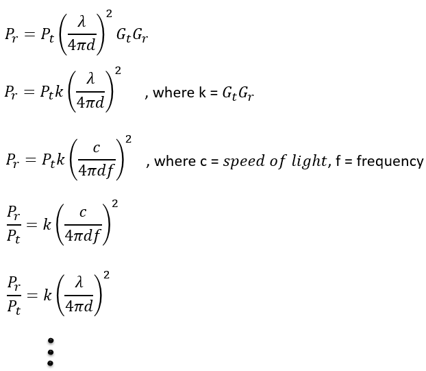
Most of these forms separate the antennas from the path. The part (λ/4πd)² is the free space path loss between two isotropic antennas. In dB, with d in km and f in MHz, it becomes FSPL = 20log₁₀(d) + 20log₁₀(f) + 32.44 dB. This is the form most link budgets use.

Let's put numbers into it. Take f = 2 GHz and d = 1 km. The path loss is 0 + 66.02 + 32.44 = 98.5 dB. A base station transmits Pt = 43 dBm into an antenna of Gt = 15 dBi, and the UE antenna has Gr = 0 dBi. The received power is then 43 + 15 + 0 - 98.5 = -40.5 dBm. Every term in this sum is one of the bullets above.

The frequency term needs one warning. The equation says that the received power falls with f², but only when Gt and Gr stay the same. An antenna of fixed physical area has a gain of 4πA/λ², so its gain rises with f². If both antennas keep their size, the two gains together rise with f⁴, and the link improves at a higher frequency. This is why millimeter wave systems use large antenna arrays. The loss at high frequency comes from the fixed gain assumption, not from space itself.

• In dB every factor is a separate term : power and gains add, and the path loss subtracts.
• FSPL = 20log₁₀(d) + 20log₁₀(f) + 32.44 dB : with d in km and f in MHz, 1 km at 2 GHz gives 98.5 dB.
• The frequency penalty depends on the antennas : it applies to fixed gains, and it reverses for antennas of fixed area.

How far can a link reach ?

The title of this page asks about radio range, so let's turn the equation around. Instead of the received power at a given distance, we ask for the distance at which the received power falls to the receiver sensitivity.

Rule of Thumb

• 6 dB improvement --> Twice the distance
• double the frequency --> half the range

Both rules come straight from the equation. The distance enters as 20log₁₀(d), and 20log₁₀(2) = 6.02 dB. So 6 dB more margin doubles the distance, and 6 dB less halves it. The frequency enters in the same way, so doubling the frequency costs 6 dB and halves the range, again for fixed antenna gains.

Solving the equation for d gives the free space range: d = (λ/4π) x 10^{(Pt + Gt + Gr - Pr,min)/20}, with all powers and gains in dB and Pr,min the receiver sensitivity. Let's use the example link above with a sensitivity of -100 dBm. The link has 43 + 15 + 0 + 100 = 158 dB to spend, and the result is about 950 km. No cellular link reaches that far. The answer is still correct for free space, and that is exactly the warning.

A real link loses power faster than free space. Ground reflection, buildings and foliage make the received power fall roughly as dⁿ, with a path loss exponent n larger than 2 in most terrestrial links. With n = 4, 6 dB more margin extends the range by only 10^6/40, about 1.41 times, instead of 2 times. So the Friis range is an upper bound. For real planning, the same link budget is used with a path loss model instead of free space. See Path Loss Model in Free Space in Fading for how the free space model sits among the others.

• 6 dB of margin doubles the free space range : because 20log₁₀(2) = 6.02 dB.
• The Friis range is an upper bound : the example link reaches about 950 km in free space, far beyond any real cell.
• Real links need a path loss exponent : with n = 4, 6 dB extends the range by only about 1.41 times.