My own image for a matrix is a kind of machine that is doing things as follows. As you see in the illustration, Matrix is taking in a shape (geometrical shape/object) and transform (change shape) them in mainly three different way as follows.

i) Scale (magnify or shrink)

ii) Rotate

iii) Skew

In reality, a matrix can do more than one type of transformation like "Scale and Skew", "Scale and Rotate and Skew" etc.

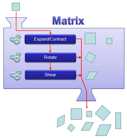
Figure 1. A matrix as a transformation machine. A square goes in, and it comes out scaled, rotated, sheared, or changed by a combination of these.

On this page the square is a grid of dots, and the machine is a 2 x 2 matrix. Instead of looking inside the machine, we'll read three numbers from the matrix and use them to predict the output shape. The six examples then show how good that prediction is.

• What can eigenvalues and the determinant tell you about a transformation ?
• How is each example generated ?
• What do the six examples show ?
• Where do these rules of thumb stop working ?

What can eigenvalues and the determinant tell you about a transformation ?

In this sections, I will show you how a matrix transforms a given image (a set of dots). For each example, I transformed 121 dots.. it means that I had to calulate "A x v" type of vector multiplication 121 times. It would have been almost undoable if I had to do it with pen and paper unless I had an extraordinary patience. (Definately I am not such a patient person -:)). Fortunately, I have a software with which I can do this kind of things relatively easy. Following is the source script that I created for these examples.  You can apply whatever 2 x 2 matrix just by changing "tm = [1.0 0.0;0.5 1.0]" part.

There are other very important points in these examples. For each example, I (matlab source script) calculated the following values and I put down a short comments on what kind of information you can get from these values.

i) Eigenvalue

ii) Angle of each Eigenvalue

iii) Determinant

When you were learning Eigenvalue, Determinant.. the first question you might have would be "What are these for ?" "Why do we have to calculate these values ?". This is one of the examples in which you can use eigenvalues and determinant in very useful way.

If there is no computer and I am asked to get overall image of the transformation of 121 points as in this example, I would definitely calculate eigenvalue and determinant and make a reasonable guess of the final result, rather than trying to 121 times of "A x v" calculation.

This kind of interpretation of Eigenvalue and Determinant is not only for geometrical transformation, but also can be useful almost any system represented as a Matrix system (e.g, Control System, Stochastics, Structure Analysis etc). So I strongly recommend you to go through in very detail and try a lot of example matrix with the Matlab/Octave script and get some intuitive understandings of your own.

NOTE : I also put some of other examples showing it in more intuitive ways at www.slide4math.com. Check [Matrix Real] section.

Here is what each of the three values tells you. An eigenvalue λ belongs to an eigenvector v, which is a direction with Mv = λv. Points along that direction are only stretched by λ, and they are never turned. The angle of an eigenvalue is 0 for a positive real value. A nonzero angle means that no real direction stays unturned, and this is the signature of a rotation. The determinant is the factor by which the area of the dot pattern changes.

There is also a link between the values. The determinant is always the product of the eigenvalues. So once you know the eigenvalues, the area factor follows, and every example below confirms it.

• Eigenvalues give the stretch along the unturned directions : a value of 1.2 means points on that eigenvector move 1.2 times farther from the origin.
• A nonzero eigenvalue angle signals rotation : complex eigenvalues come in pairs with angles +θ and -θ.
• The determinant is the area factor : above 1 the pattern grows, below 1 it shrinks, and at 1 its area stays the same.
• The three numbers predict the picture : you can guess the output before computing a single product.

How is each example generated ?

Every figure on this page comes from one short script, and only the matrix tm changes between them. The script is given twice, for GNU Octave and for Matlab. You can paste either one and replace tm with any 2 x 2 matrix you want to explore.

Octave Code

This version runs in GNU Octave. It builds the grid of dots, applies tm, prints the eigenvalues, their angles and the determinant, and plots the dots before and after. Its tm is the shear of Figure 6.

ptList_x=[];
ptList_y=[];

for y=-1.0:0.2:1.0
for x=-1.0:0.2:1.0
    ptList_x=[ptList_x x];
    ptList_y=[ptList_y y];
end
end

ptList_v = [ptList_x' ptList_y'];
ptList_v = ptList_v';

tm = [1.0 0.0;0.5 1.0]
tm_eigenvalue = eig(tm)
Angle_of_eigenvalues = arg(tm_eigenvalue)
tm_determinant = det(tm)

ptList_v_tm = tm * ptList_v;
ptList_v_tm_x = ptList_v_tm(1,:);
ptList_v_tm_x = ptList_v_tm_x';
ptList_v_tm_y = ptList_v_tm(2,:);
ptList_v_tm_y = ptList_v_tm_y';

subplot(1,2,1);
plot(ptList_x,ptList_y,'ro','MarkerFaceColor',[1 0 0]);axis([-2 2 -2 2]);title('x');daspect([1 1]);
subplot(1,2,2);
plot(ptList_v_tm_x,ptList_v_tm_y,'bo','MarkerFaceColor',[0 0 1]);axis([-2 2 -2 2]);title('tm.x');daspect([1 1]);

Matlab Code

This version runs in Matlab. It is the same script with angle() in place of arg() and axis square in place of daspect. Its tm is the shear of Figure 5, [1.0 0.5; 0.0 1.0].

ptList_x=[];
ptList_y=[];

for y=-1.0:0.2:1.0
for x=-1.0:0.2:1.0
    ptList_x=[ptList_x x];
    ptList_y=[ptList_y y];
end
end

ptList_v = [ptList_x' ptList_y'];
ptList_v = ptList_v';

tm = [1.0 0.5;0.0 1.0]
tm_eigenvalue = eig(tm)
Angle_of_eigenvalues = angle(tm_eigenvalue)
tm_determinant = det(tm)

ptList_v_tm = tm * ptList_v;
ptList_v_tm_x = ptList_v_tm(1,:);
ptList_v_tm_x = ptList_v_tm_x';
ptList_v_tm_y = ptList_v_tm(2,:);
ptList_v_tm_y = ptList_v_tm_y';

subplot(1,2,1);
plot(ptList_x,ptList_y,'ro','MarkerFaceColor',[1 0 0]);axis([-2 2 -2 2]);
title('x');axis square;
subplot(1,2,2);
plot(ptList_v_tm_x,ptList_v_tm_y,'bo','MarkerFaceColor',[0 0 1]);axis([-2 2 -2 2]);
title('tm.x');axis square;

The two loops run x and y from -1.0 to 1.0 in steps of 0.2. That gives 11 values per axis, so the grid holds 11 x 11 = 121 dots. The matrix ptList_v stores one dot per column. So the single line ptList_v_tm = tm * ptList_v does all 121 matrix-vector products at once. The functions arg() and angle() both return the angle of a complex number in radians, which is the unit of the angles printed in the figures.

• Change only tm : the rest of the script stays the same for any 2 x 2 matrix.
• One matrix product moves every dot : stacking the dots as columns replaces a loop over 121 points.
• Angles are in radians : 0.5236 rad is 30 deg.

What do the six examples show ?

Each figure below applies one 2 x 2 matrix M to the same square of dots. The red dots are the input, and the blue dots are M times each red dot. The notes on the right of each figure read the three values printed at the lower left. Try to predict each blue pattern from the three values before you look at it.

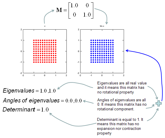
Figure 2. The identity matrix. Both eigenvalues are 1, both angles are 0 and the determinant is 1, so nothing changes.

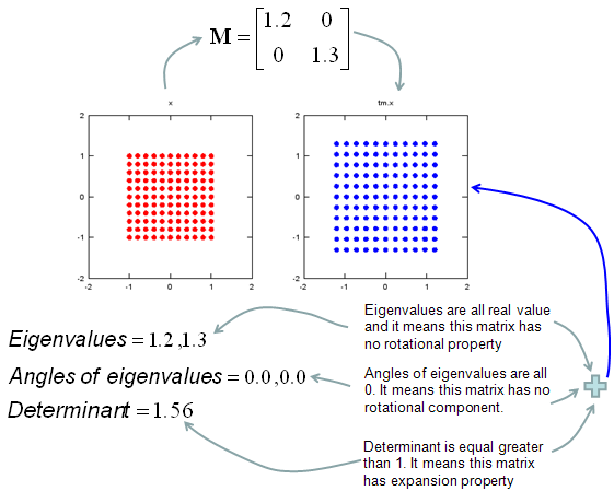
Figure 3. A diagonal matrix with 1.2 and 1.3. The square stretches by 1.2 along x and by 1.3 along y, and its area grows by 1.2 x 1.3 = 1.56.

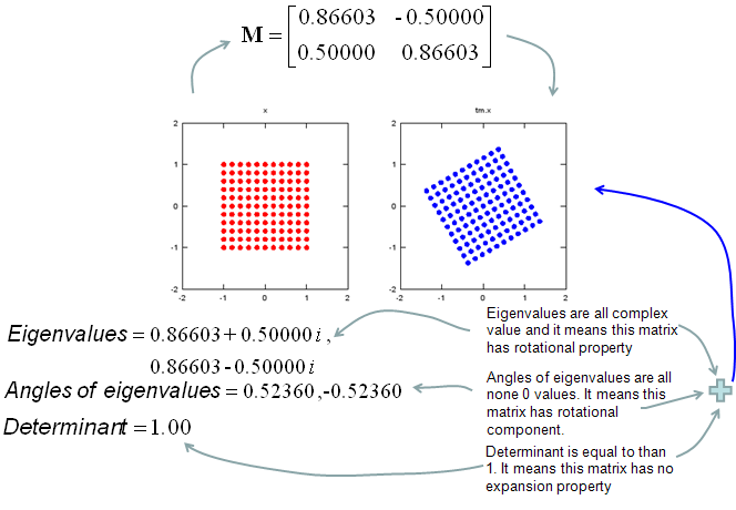
Figure 4. A rotation by 30 deg. The eigenvalues are complex, their angles are +/-0.5236 rad, and the determinant is 1.

The rotation in Figure 4 is counterclockwise, because the matrix has the form [cos θ -sin θ; sin θ cos θ] with θ = 30 deg. The angle of the eigenvalues, 0.5236 rad, is exactly this rotation angle. The note in the figure says the determinant is equal to than 1, which should read equal to 1.

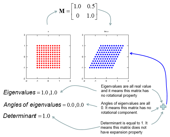
Figure 5. A horizontal shear. The eigenvalues are 1 and 1 and the determinant is 1, so the area stays the same while the square leans.

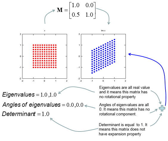
Figure 6. A vertical shear. The values are the same as for the horizontal shear, but the square leans upward instead of sideways.

Figure 5 and Figure 6 have identical eigenvalues, angles and determinants, but different pictures. So the three values cannot tell you the direction of a shear. For that you need the eigenvectors. The only eigenvector direction of the horizontal shear is the x axis, and the only one of the vertical shear is the y axis.

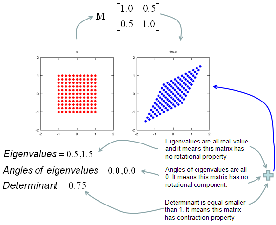
Figure 7. A symmetric matrix. The pattern stretches by 1.5 along the (1, 1) diagonal and shrinks to 0.5 across it, so the area factor is 0.75.

The table below collects the six examples. The note in Figure 3 says the determinant is equal greater than 1, which should read greater than 1. In every row, the determinant equals the product of the two eigenvalues.

• Real eigenvalues with angle 0 : the pattern is stretched or sheared, but not rotated as a whole.
• Complex eigenvalues : the whole pattern turns, and the angle shows by how much for a pure rotation.
• Determinant 1 : the area stays the same, as in the rotation and the two shears.
• Same values, different picture : the eigenvectors decide the direction in which the pattern stretches or leans.

Where do these rules of thumb stop working ?

The notes inside the figures are good rules of thumb, but two of them claim more than the mathematics allows. Knowing where they stop working keeps you from misreading a new matrix. Let's test each rule with the examples above.

First, real eigenvalues do not mean that no point turns. They mean that at least one direction is only stretched and not turned. Take the shear of Figure 5. Its eigenvalues are 1 and 1, but the point (0, 1) goes to (0.5, 1), so it clearly turns. Only the points on the x axis keep their direction. In Figure 7, the eigenvectors lie along (1, 1) and (1, -1). Every other point turns toward the (1, 1) diagonal, because that direction is stretched by 1.5 while the other shrinks to 0.5.

Second, the angle of an eigenvalue equals the visible turn only for a pure rotation, as in Figure 4. A matrix that rotates and stretches unequally also has complex eigenvalues. Their angle then signals rotation, but different points turn by different amounts. Also note that an angle of π is a rotation too. The matrix [-1 0; 0 -1] turns every point by 180 deg, and its eigenvalues are the real number -1. Their angle is π, not 0, so the angle rule still catches it.

Third, the determinant measures area, not length. In Figure 7 the determinant is 0.75, and the note calls this a contraction. Yet the pattern grows by 1.5 along the (1, 1) diagonal. It shrinks by 0.5 across it, and 1.5 x 0.5 = 0.75. So only the area shrinks. Finally, a negative determinant means the pattern is mirrored, and a zero determinant means all the dots collapse onto one line. You can see both cases with tm = [-1 0; 0 1] and tm = [1 2; 0.5 1] in the script.

• Real eigenvalues guarantee one unturned direction : they do not stop other points from turning.
• The eigenvalue angle is exact only for a pure rotation : and an angle of π means a half turn.
• The determinant is an area factor : a shape can shrink in area while it grows in one direction.
• Check the sign of the determinant : a negative value means a mirror image, and 0 means a collapse onto a line.