LDPC stands for "Low-Density Parity-Check". It's a method used in communication systems for encoding and decoding data to detect and correct errors. LDPC codes are a type of linear error-correcting code that has found extensive application in modern communication technologies. LDPC codes are a powerful and efficient method for error correction in digital communication systems, enabling reliable data transmission even in challenging and noisy environments.
Here are some key points about LDPC:
Error Correction : LDPC codes are particularly effective for correcting data transmission errors in noisy communication channels. They are used in scenarios where accurate data transmission is critical, such as in satellite communication, wireless networks, and data storage.Sparse Parity-Check Matrix : The 'low-density' in LDPC refers to the parity-check matrix used in these codes, which has a relatively small number of non-zero elements. This sparsity is what makes LDPC codes computationally efficient for error correction.Decoding Algorithm : LDPC codes are usually decoded using iterative probabilistic decoding algorithms, such as the belief propagation (BP) algorithm. These algorithms are efficient and can handle a large number of errors.Applications : LDPC codes are widely used in modern communication standards, including Wi-Fi (as part of the IEEE 802.11 standard), 5G cellular networks, and digital television (DVB-T2 and DVB-S2).History and Development : LDPC codes were first introduced by Robert G. Gallager in his doctoral dissertation at MIT in 1960. However, they were not widely used until the 1990s when advancements in digital technology made their implementation more feasible.Performance : LDPC codes are known for their near-Shannon-limit performance. The Shannon limit is a theoretical maximum efficiency for data communication in a channel with a given level of noise.
This note is about LDPC with the perspective of the implementation in 5G/NR. Followings are the topics to be covered in this note
- What I did to understand this ?
- LDPC in NR
- What is QC-LDPC?
- What is Lifting ?
- LDPC Encoding
- LDPC Decoding
- Why LDPC is Compute-Intensive ?
What I did to understand this ?
As almost everybody would agree, LDPC is one of the most mysterious concepts in the NR specification.
Even though the algorithm itself has existed for a very long time, I think there are not many people who have seriously tried to understand all the technical details behind it. Many people may know that NR uses LDPC for data channel coding. Many people may also know some keywords such as parity check matrix, Tanner graph, base graph, and lifting size. But connecting all of these into one clear picture is not easy. The following is not a dry technical description of LDPC. It is more like a record of how my understanding evolved step by step. It shows the phases I personally went through from the beginning until I reached my current level of understanding.
- Phase 1 : Read 3GPP specification and try to decode the meaning out of the text. Of course, make NO SENSE AT ALL to me
- Phase 2 : Read some background technical documents about the high level concept. I just picked some key words like 'Density', 'Parity', 'Graph' etc. But NO CONNECTED DOTS and No idea on how those concepts are associated with description in 3GPP spec
- Phase 3 : I came up with describing LDPC in a very simple math equation H c = 0. Then the question came up. In this equation, which one is known and which one is unknown ?
- Phase 4 : After leaning that H is known, I came up with question : How H matrix is constructed in 3GPP ?
- Phase 5 : Constructing H matrix and c vector in code (javascript) for interactive simulation.
Phase 1 : Read 3GPP specification and try to decode the meaning out of the text. Of course, make NO SENSE AT ALL to me
My first approach was very simple.
I opened the 3GPP specification and tried to understand LDPC directly from the text.
At that time, I thought this would be the most reliable way. Since the specification is the final authority, I assumed that careful reading would eventually explain everything.
But it did not work that way.
The specification showed many tables, parameters, indexes, and pseudo-code like descriptions. I could see that they were describing some kind of channel coding procedure. But I could not build a clear picture in my mind.
I already had some high-level understanding of channel coding. I knew basic ideas of convolutional coding, turbo coding, and block coding. But LDPC did not clearly fall into any of those familiar pictures for me.
So the first confusion was very basic.
- Is LDPC just another kind of block coding ?
- Is it similar to turbo coding ?
- Is it completely different ?
Why does the specification talk so much about matrices, base graphs, lifting size, and circular shifts ?
At this stage, I was not really learning LDPC yet.
I was mostly realizing that reading the specification alone was not enough. The specification tells us what to do. But it does not always tell us how to think about it.
That was the first important lesson.
Before decoding the LDPC algorithm, I first had to decode the way LDPC is described.
Phase 2 : Read some background technical documents about the high level concept. I just picked some key words like 'Density', 'Parity', 'Graph' etc. But NO CONNECTED DOTS and No idea on how those concepts are associated with description in 3GPP spec
After failing to understand LDPC directly from the 3GPP specification, I changed my approach.
I started reading background technical documents about LDPC. My expectation was that these documents would explain the high-level concept first, and then I would be able to go back to the 3GPP specification with a clearer picture.
At this stage, I learned that LDPC stands for Low Density Parity Check Code.
The name itself gave me some hints.
Low density seemed to mean that the matrix is sparse. In other words, the matrix has many zeros and only a small number of ones. Parity was also a familiar word. I had seen parity in basic computer science, and also in communication technology such as RS232. So I thought I had at least some rough feeling about the meaning.
But still, the full picture was not clear.
Then I started seeing another important word again and again.
One of the new term that caught my attention was Graph.
Many LDPC explanations talked about graphs, nodes, edges, variable nodes, check nodes, and Tanner graphs. I could understand each word separately at a very shallow level. But I could not connect them together.
- Is this graph the same kind of graph used in graph theory ?
- How is this graph related to the parity check matrix ?
- Why does a channel coding problem suddenly become a graph problem ?
- How does this graph help the receiver recover the original data ?
These words looked important, but they were still scattered words.
- Density was one word.
- Parity was another word.
- Graph was another word.
- Matrix was another word.
But there were no connected dots yet.
I still could not see how these concepts were related to the actual description in the 3GPP specification. The specification talked about base graph, lifting size, shift values, and matrix expansion. The background documents talked about sparse matrices and Tanner graphs.
I could sense that they were talking about the same thing from different angles. But I could not yet see the bridge between them.
So Phase 2 was useful, but it was still frustrating.
I collected many keywords. But I did not yet have one single mental picture that could connect all of them.
Phase 3 : I came up with describing LDPC in a very simple math equation H c = 0. Then the question came up. In this equation, which one is known and which one is unknown ?
After collecting many scattered keywords, I needed something simpler.
So I learned a basic equation to describe the concept of LDPC.
H c = 0
At first, this looked too simple.
But this simple equation created the first real question for me.
- In this equation, which one is known and which one is unknown ?
- Is H something that the receiver has to discover ?
- Is c the original transmitted data ?
- Is c the received data ?
- Or is c the final codeword that the receiver is trying to recover ?
This question was important because I realized that I was not even clear about the role of each element.
- If I do not know what H means, I cannot understand the parity check matrix.
- If I do not know what c means, I cannot understand what the decoder is checking.
- If I do not know which one is known and which one is unknown, I cannot understand what decoding is trying to do.
Then the picture started to become a little clearer.
- H is the known structure.
- It defines the parity check rules.
- c is the codeword that should satisfy those rules.
- If c is a valid codeword, then multiplying it by H should produce zero. That zero does not mean all data bits are zero. It means all parity check rules are satisfied.
This was a small step, but it was an important turning point. LDPC was no longer just a mysterious set of tables in the specification.
It started to look like a question: : "Given a known rule H, can we find a codeword c that satisfies H c = 0, even when the received signal is noisy ?"
Phase 4 : After leaning that H is known, I came up with question : How H matrix is constructed in 3GPP ?
After I understood that H is known, the next question naturally came up.
If H is known, where does it come from ?
At first, I thought H may be given as one big matrix. In a textbook example, this is usually possible. The parity check matrix can be shown directly with zeros and ones. Then we can multiply H and c and check whether the result becomes zero.
But NR LDPC is not that simple.
The matrix is too large to write directly. Also, the matrix is not always the same. It changes depending on the transport block size, code rate, base graph, lifting size, and other parameters.
So 3GPP does not simply say, “Here is the H matrix”. Instead, 3GPP describes how to construct H.
This was another important turning point for me.
H is known, but it is not stored as one fixed matrix. It is generated from a smaller structure.
Then new questions started appearing.
- What is a base graph ?
- Why are there two base graphs ?
- What is lifting ?
- What does lifting size mean ?
- Why does one small entry in the base graph become a larger shifted identity matrix ?
- What does the shift value mean ?
- Why does -1 mean an all-zero matrix ?
- How does this small base graph become the huge parity check matrix used for real decoding ?
At this stage, I realized that understanding LDPC in NR is not just about understanding the equation H c = 0.
I also had to understand how NR creates H before using that equation.This is where the 3GPP tables started to look a little different.
At first, those tables looked like random numbers. But later, I started to see them as construction instructions.
- They are not just numbers.
- They are telling the receiver how to build the parity check structure.
- They are telling which parts are connected.
- They are telling how the small base graph is expanded into the real H matrix.
So Phase 4 changed my question again.
The question was no longer only: What is H ?
The new question became: How does 3GPP generate H from base graph, lifting size, and shift values ?
Phase 5 : Constructing H matrix and c vector in code (javascript) for interactive simulation.
This was the phase that gave me the clearest and most concrete understanding of 3GPP LDPC.
Until this point, I had learned many concepts.
- I learned that H is known.
- I learned that c should satisfy H c = 0.
- I learned that H is not written directly as one huge matrix in 3GPP.
- I learned that it is constructed from base graph, lifting size, and shift values.
But still, the understanding was not fully concrete. Then I started implementing it in code. I tried to construct the H matrix by myself. I also created a c vector and tested whether the equation H c = 0 really works.
This changed the feeling completely.
- The base graph was no longer just a table in the specification.
- The lifting size was no longer just a parameter.
- The shift value was no longer just a number.
- I could see how each entry in the base graph expands into a small matrix.
- I could see how -1 becomes an all-zero block.
- I could see how other values become circularly shifted identity matrices.
- I could see how all of these blocks are connected together to form the final H matrix.
This was the moment when 3GPP LDPC started to look real to me.
Before coding, I was mostly reading and imagining.
After coding, I could actually see the structure being created.
I used JavaScript because I wanted to make it interactive. I wanted to change parameters, generate the matrix, create vectors, and observe the result directly.
This was not just an implementation exercise. It was a learning tool.
By constructing H and c in code, I could finally connect the equation, the graph, and the 3GPP tables into one picture.
If you are interested in what I've implemented using AI, check this out.
LDPC in NR
NR selected LDPC for the data channels (PDSCH and PUSCH ) due to its excellent performance and suitability for high-throughput, parallel processing.
High Level Procedure of LDPC Encoding
This is about LDPC encoding process at the very highlevel based on my own understanding.
This procedure shows that NR LDPC encoding is not a single fixed code. It is a structured family of codes. The encoder first treats the transport block as the input constraint. It then chooses the LDPC “template” that best fits that constraint, so the same physical mechanism can support very different TBS and code-rate points without redefining the whole parity-check matrix every time.
The key idea is the separation between a small base graph and a large practical matrix. The base graph is the high-level structure that defines how variable nodes and check nodes are connected. Once the base graph is decided, the encoder does not build a brand-new design from scratch. It “lifts” the base graph by a lifting size, so each base-graph entry expands into a block made of circularly shifted identity matrices. This is how the final H matrix becomes large enough for real payload sizes while keeping the structure regular and implementation-friendly.
After that, encoding becomes a constraint satisfaction problem in a very concrete form. You are looking for a codeword vector c that makes all parity checks pass, which is expressed as H · c = 0. So the whole flow can be viewed as: pick the right structural template for the target operating point, scale it up using a standardized lifting rule, and then generate parity bits so the resulting codeword satisfies the parity-check equations.
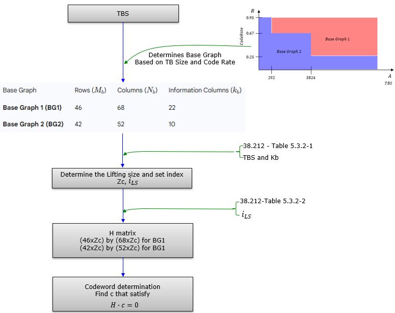
Now let me verbalize this diagram and it goes as follows
- Overall flow (what the diagram is trying to teach)
- Start from a payload requirement (TBS) and a protection requirement (code rate)
- Choose a standardized LDPC “template” (Base Graph)
- Scale that template to the exact needed size (Lifting)
- Build the parity-check matrix H from the lifted structure
- Encode by finding a codeword c that satisfies the parity constraints
- 1) Input: TBS
- TBS is the anchor parameter
- It represents the amount of transport data to be protected by LDPC
- TBS is used together with code rate
- Because “small vs large block” and “low vs high rate” drive different best structures
- TBS is the anchor parameter
- 2) Base Graph selection (BG1 vs BG2)
- Base Graph is selected based on TBS and code rate
- The figure emphasizes a region split where BG2 tends to cover smaller / different rate regions and BG1 covers larger / other regions
- The Base Graph defines the mother structure size
- BG1 has its own (Mb, Nb, kb)
- BG2 has its own (Mb, Nb, kb)
- Practical meaning
- This step decides the “shape” of the LDPC code before any scaling happens
- Base Graph is selected based on TBS and code rate
- 3) Lifting decision (Zc, iLS)
- Once BG is fixed, choose the lifting size
- Zc is the expansion factor
- Choose the lifting set index
- iLS selects which standardized lifting size entry is used
- Practical meaning
- This step turns “one base template” into “many usable code sizes” in a controlled way
- Once BG is fixed, choose the lifting size
- 4) Construct the full parity-check matrix H
- Build H by lifting the base graph
- Each base-graph entry expands into a Zc × Zc block
- Either a zero block or a shifted-identity type block
- Each base-graph entry expands into a Zc × Zc block
- Resulting matrix dimensions scale with Zc
- For BG1: (46 · Zc) × (68 · Zc)
- For BG2: (42 · Zc) × (52 · Zc)
- Practical meaning
- The base graph gives the pattern, lifting gives the real size
- Build H by lifting the base graph
- 5) Codeword determination (encoding constraint)
- Encoding is framed as satisfying parity checks
- Find codeword c such that H · c = 0
- Practical meaning
- Parity bits are chosen so the final vector lies in the valid LDPC code space defined by H
- Encoding is framed as satisfying parity checks
Core Principle - Sparsity
Simply put, the final goal of LDPC is to find out parity bits that satisfy the following equation: H × cT = 0 (modulo 2). This equation is the foundation of Low-Density Parity-Check (LDPC) codes, ensuring that a codeword c adheres to the parity-check constraints defined by the parity-check matrix H. The example in the image illustrates this principle through the encoding process, where the objective is to compute parity bits p given information bits s, such that the resulting codeword c satisfies this equation. Let’s elaborate on this as the core principle of LDPC, particularly in the context of 3GPP’s 5G NR, and explore its broader significance.
- LDPC codes are defined by a parity-check matrix (H). This matrix is "low-density," meaning it contains very few '1's and mostly '0's.
- Each row in H represents a parity-check equation, which is a simple XOR sum of a subset of the transmitted bits (codeword bits) that must equal zero for a valid codeword.
- Each column corresponds to a specific bit in the codeword.
- The sparsity is crucial because it allows for efficient iterative decoding algorithms.
As a simple example, let's assume that we have a data s = [s1, s2, s3, s4] = [1, 0, 1, 1], meaning there are 4 bits of data (k = 4) and want to encode this to a codeword c = [s1, s2, s3, s4, p1, p2, p3, p4]. The final goal of LDPC is to find the p1, p2, p3, p4 to meet the condition H × cT = 0 (modulo 2).
The complicated part of LDPC in real application (as in 5G) is about how to construct H matrix and How to decode the received LDPC data into original message.
You're asking an interesting question about modifying the fundamental condition of LDPC codes from H × cT = 0 to H × cT = 1. Let’s explore why this change would not work in the context of LDPC codes, particularly as they are implemented in 3GPP’s 5G NR, and what the practical implications would be.
Understanding the Standard Condition: H × cT = 0
In LDPC codes (and linear block codes in general), the condition H × cT = 0 (with operations in GF(2), i.e., modulo 2) ensures that the codeword c satisfies all parity-check equations defined by the parity-check matrix H. This condition is fundamental for several reasons:
- Parity Checks: Each row of H represents a parity-check equation. For example, if a row of H has 1s in positions 1, 3, and 5, the corresponding equation is c1 + c3 + c5 = 0, meaning the sum of those bits (modulo 2) must be 0 (an even number of 1s).
- Error Detection: At the receiver, if H × rT ≠ 0 for a received vector r, it indicates errors, and the decoder uses this to correct them.
- Systematic Structure: The condition allows for systematic encoding, where the codeword c contains the original information bits plus parity bits that make the parity checks hold.
This setup ensures that the code has a well-defined structure, enabling efficient encoding, decoding, and error correction.
What Happens If We Change to H × cT = 1?
If we redefine the condition to H × cT = 1, we’re fundamentally altering the rules of the code. Let’s break down why this wouldn’t work:
-
Inconsistency with Linear Code Theory
- Linear Codes: LDPC codes are linear block codes, meaning the set of valid codewords forms a vector space (a subspace of {0,1}n). For a linear code, the all-zero codeword c = [0, 0, …, 0] must always be a valid codeword because it trivially satisfies H × 0T = 0.
- With H × cT = 1:
- If c = [0, 0, …, 0], then H × 0T = 0, which does not equal 1. So, the all-zero codeword would not be valid.
- This violates the linearity property, as the set of codewords would no longer form a vector space (since the zero vector is not included).
- Practical Impact: Linearity is crucial for efficient encoding and decoding. Without it, many standard algorithms (like syndrome decoding or belief propagation in LDPC) would break down.
-
Inconsistent Parity Checks
- Standard Case (H × cT = 0): Each row of H enforces a parity check where the sum of the bits (where H has 1s) must be even (0 modulo 2). For example, if a row of H is [1, 0, 1, 0, 1, 0, 0, 0], the equation is c1 + c3 + c5 = 0.
- Modified Case (H × cT = 1): Now, each row would require the sum of the bits to be odd (1 modulo 2). For the same row, the equation becomes c1 + c3 + c5 = 1.
- Problem: If H has m rows, then H × cT = 1 means every parity check must result in 1 (an odd sum). This creates a highly constrained system:
- The equations may not have a solution for all input data. For example, if two rows of H are identical (e.g., both enforce c1 + c3 + c5 = 1), they cannot both be satisfied simultaneously because they would require the same sum to be both odd and odd, but there’s only one sum.
- In general, the system of equations H × cT = [1, 1, …, 1]T (an all-1 vector of length m) is over-constrained and often has no solution, especially if the rows of H are not carefully designed to ensure solvability.
-
Encoding Becomes Infeasible
- Standard Encoding: In LDPC (e.g., in 3GPP), we compute parity bits to satisfy H × cT = 0. This is straightforward because the equations are homogeneous (equal to 0), and we can solve for the parity bits systematically.
- Modified Encoding: With H × cT = 1, the equations become non-homogeneous (equal to 1). Solving for parity bits becomes much harder:
- The system H × cT = [1, 1, …, 1]T may not have a solution, as mentioned above.
- Even if a solution exists, it may not be unique, leading to ambiguity in encoding.
- Practical Impact: In 3GPP, encoding needs to be fast and deterministic for high-throughput applications (e.g., 5G’s multi-Gbps rates). An unsolvable or ambiguous system would make encoding impractical.
-
Decoding Breaks Down
- Standard Decoding: LDPC decoding (e.g., Belief Propagation) relies on the syndrome H × rT. If H × rT = 0, the received vector r is a valid codeword. If not, the non-zero syndrome guides the iterative correction process.
- Modified Decoding: If the goal is H × rT = 1, the decoding process becomes problematic:
- The syndrome would be computed as H × rT ⊕ [1, 1, …, 1]T, but the iterative message-passing algorithms (like Belief Propagation) are designed for the H × cT = 0 framework.
- The Tanner graph (used for decoding) assumes that check nodes enforce even parity (sum = 0). Changing this to odd parity (sum = 1) for all checks disrupts the algorithm’s convergence properties.
- Practical Impact: In 5G NR, decoding must be efficient and reliable. The modified condition would make error correction either impossible or extremely inefficient.
-
Loss of Error Detection Capability
- Standard Case: If a received vector r has errors, H × rT ≠ 0, and the non-zero syndrome helps identify and correct errors.
- Modified Case: If the goal is H × rT = 1, the syndrome check becomes H × rT ≟ [1, 1, …, 1]T. But since the system is often unsolvable, it’s unclear how to interpret deviations from this condition, making error detection and correction unreliable.
Could It Work in a Different Context?
The condition H × cT = 1 resembles a non-homogeneous system, which isn’t typical for linear block codes but could be interpreted in other coding schemes:
- Affine Codes: Instead of a linear code (where the codewords form a vector space), you could define an affine code, where the codewords are an affine subspace (a linear subspace shifted by a fixed vector). This would mean H × cT = b, where b is a fixed non-zero vector (e.g., [1, 1, …, 1]T). However:
- This is not how LDPC codes are defined in 3GPP or in standard practice.
- It loses the benefits of linearity, making encoding and decoding much harder.
- Modified Parity Checks: You could design a code where some parity checks result in 1 instead of 0, but this would require a different H matrix and a modified decoding algorithm, which isn’t compatible with standard LDPC frameworks like those in 5G NR.
Practical Implications in 3GPP
In 3GPP’s 5G NR, LDPC codes rely on H × cT = 0 for:
- Efficient Encoding: The quasi-cyclic structure of H (using base graphs and lifting) allows fast computation of parity bits.
- Reliable Decoding: Iterative decoding (Belief Propagation) is optimized for the H × cT = 0 condition, ensuring high throughput and low error rates.
- Error Detection: The syndrome check H × rT = 0 is critical for detecting and correcting errors in noisy channels.
Changing to H × cT = 1:
- Breaks the linearity of the code, making standard LDPC algorithms unusable.
- Makes encoding and decoding infeasible or inefficient, which is unacceptable for 5G’s high-speed, reliable communication requirements.
- Disrupts the entire error correction framework, leading to unreliable data transmission.
Summary
The condition H × cT = 1 would not work for LDPC codes as defined in 3GPP or in standard practice because:
- It violates the linearity of the code, breaking fundamental properties.
- It creates an over-constrained system that often has no solution, making encoding impossible.
- It disrupts standard decoding algorithms, rendering error correction inefficient or infeasible.
- It loses the practical benefits (efficiency, reliability) that make LDPC codes suitable for 5G NR.
The H × cT = 0 condition is not arbitrary—it’s a cornerstone of linear block codes like LDPC, ensuring they are practical and effective for real-world communication systems. If you’d like to explore alternative coding schemes where non-homogeneous conditions might apply, let me know!
LDPC Implementation in 5G - Structure
- Quasi-Cyclic LDPC (QC-LDPC): 3GPP uses a specific structure called QC-LDPC. This structure makes hardware implementation much more efficient and manageable. The large parity-check matrix (H) is constructed from smaller sub-matrices which are either zero matrices or circulant permutation matrices (identity matrices with columns cyclically shifted).
- Base Graphs (BG): 3GPP defines two fundamental Base Graphs, BG1 and BG2.
- BG1: Designed for larger data blocks and generally higher code rates.
- BG2: Designed for smaller data blocks and generally lower code rates.
- The choice between BG1 and BG2 depends on the transport block size and the target code rate.
- Lifting: The actual parity-check matrix used for encoding/decoding is generated by "lifting" the selected Base Graph (BG1 or BG2). This involves replacing each '1' in the base graph matrix with a specific circulant permutation matrix (based on shifts defined in the standard) of size ZxZ, and each '0' with a ZxZ zero matrix. The value 'Z' is called the lifting size, and it's chosen from a set of predefined values based on the required code block length. This lifting process creates the larger, final QC-LDPC parity-check matrix H.
- Code Block Segmentation: If a transport block (the data coming from higher layers) is very large, it's first segmented into smaller code blocks. A CRC (Cyclic Redundancy Check) is added to each code block before LDPC encoding. Each code block is then encoded independently using LDPC. This limits the maximum complexity of the LDPC encoder/decoder.
Encoding
While LDPC codes are defined by the parity-check matrix H, encoding isn't as straightforward as with some other codes. 3GPP defines specific efficient encoding procedures based on the structured nature (QC-LDPC) of the codes. Essentially, given the information bits, the encoder calculates the necessary parity bits such that the resulting codeword (information bits + parity bits) satisfies all the parity-check equations defined by H (i.e., H * cT = 0, where c
is the codeword vector).
Rate Matching
Wireless systems need to adapt the coding rate (ratio of information bits to total transmitted bits) based on channel conditions. LDPC in 3GPP uses a flexible rate matching procedure.
- A base LDPC code (often low-rate) is generated.
- To achieve the desired code rate for transmission, some coded bits (usually parity bits, but sometimes information bits too for very high rates) are selected for transmission, while others are punctured (not transmitted) or shortened. For lower rates, bits might be repeated.
- 3GPP uses a circular buffer approach. All encoded bits (systematic/information and parity) are written into a buffer. Bits are then read out sequentially (and cyclically if needed) from this buffer for transmission, selecting the exact number of bits needed to match the allocated radio resources and target code rate.
Decoding
At the receiver, an iterative decoding algorithm is used, typically the Belief Propagation (also known as Sum-Product) algorithm or a variation like Min-Sum.
- This algorithm works on the Tanner Graph representation of the LDPC code (a bipartite graph connecting variable nodes representing codeword bits and check nodes representing parity-check equations).
- The decoder passes messages (probabilities or log-likelihood ratios) back and forth between variable nodes and check nodes along the edges of the Tanner graph.
- In each iteration, the nodes update their belief about the value of each received bit based on the messages received from their neighbours and the received signal strength for that bit.
- This process repeats for a fixed number of iterations or until the decoded bits form a valid codeword (i.e., satisfy all parity-check equations) or converge.
- The parallel nature of message passing across the sparse graph makes LDPC decoding suitable for high-speed hardware implementation.
What is QC-LDPC?
QC-LDPC is a specific type of Low-Density Parity-Check (LDPC) code where the parity-check matrix (H) has a special, structured form. Instead of being an arbitrary sparse matrix, it's constructed from smaller square blocks, each of which is either a zero matrix or a circulant permutation matrix (CPM).
Key Concepts
1. LDPC Recap: Remember that LDPC codes are defined by a sparse parity-check matrix H. A vector c is a valid codeword if H * cT = 0. Sparsity allows for efficient iterative decoding.
2. Cyclic Codes: In a strictly cyclic code, if you cyclically shift a valid codeword, you get another valid codeword. QC-LDPC is a generalization.
3. Circulant Permutation Matrix (CPM): This is the fundamental building block. A CPM is a square matrix (say, size Z x Z) where each row is a cyclic shift of the row above it. Crucially, each row and column has exactly one '1' and the rest '0's. They are essentially cyclically shifted identity matrices.
- The identity matrix (I) is a CPM (zero shift).
- A cyclically shifted identity matrix is a CPM. For example, shifting the 3x3 identity matrix
I_3right by one position gives:I3=
Shifted(1 0 0 0 1 0 0 0 1 I3, 1) =0 1 0 0 0 1 1 0 0 - The zero matrix (all zeros) is often considered trivially in this context as well, representing the absence of connections in the Tanner graph.
4. Quasi-Cyclic Structure: The "Quasi" part means the entire H matrix isn't necessarily cyclic, but it *is* composed of these CPM blocks (and zero blocks). If you divide the H matrix into ZxZ blocks, each block is a CPM or a zero matrix.
How is the H Matrix Constructed?
Often, a QC-LDPC matrix H is defined by:
1. A Lifting Factor (or Expansion Factor) Z: This defines the size (Z x Z) of the circulant blocks.
2. A Base Matrix (or Model Matrix) B: This is a smaller matrix whose entries tell you which CPM to place in the corresponding block position in the final H matrix.
- An entry
s(wheres >= 0) in the base matrix means: place the ZxZ identity matrix cyclically shifted byspositions in that block location. - A special entry (e.g., -1 or ∞, depending on convention) means: place the ZxZ zero matrix in that block location.
If the Base Matrix B has dimensions M_b x N_b, and the lifting factor is Z, the final QC-LDPC matrix H will have dimensions (M_b * Z) x (N_b * Z).
Example
Let's construct a small QC-LDPC matrix H.
Choose Lifting Factor Z = 3.
Define a Base Matrix B (size 2x4): Base Matrix refers to the matrix representation of what is called 'Base Graph' in 3GPP.
B =
| 0 | 2 | −1 | 1 |
| 1 | −1 | 2 | 0 |
This is just an example of the simple Base Matrix. This is a Base Matrix (B) used to define the structure of a Quasi-Cyclic LDPC (QC-LDPC) parity-check matrix (H).
This matrix doesn't directly contain message data. Instead, each number tells you how to construct a block within the larger, final parity-check matrix H. You need a Lifting Factor (Z) (which was Z=3 in the previous example) to interpret these numbers:
- Non-negative numbers (
0,1,2): These numbers represent a cyclic shift applied to a ZxZ identity matrix.0: Represents the ZxZ identity matrix with no shift (P0).1: Represents the ZxZ identity matrix cyclically shifted right by 1 position (P1).2: Represents the ZxZ identity matrix cyclically shifted right by 2 positions (P2).- In general, a non-negative number
srepresents the ZxZ identity matrix shiftedstimes (Ps).
- Negative number (
-1): As the text below the matrix in the image notes, the convention here is that-1represents the Z x Z zero matrix (0_Z). This means this block position in the final H matrix will consist entirely of zeros. (Sometimes other conventions like using infinity are used for the zero matrix).
Now, we need the 3x3 circulant permutation matrices corresponding to the shifts 0, 1, and 2, plus the 3x3 zero matrix:
P0 (Identity, shift 0):
| 1 | 0 | 0 |
| 0 | 1 | 0 |
| 0 | 0 | 1 |
P1 (Shift right by 1):
| 0 | 1 | 0 |
| 0 | 0 | 1 |
| 1 | 0 | 0 |
P2 (Shift right by 2):
| 0 | 0 | 1 |
| 1 | 0 | 0 |
| 0 | 1 | 0 |
03 (Zero matrix):
| 0 | 0 | 0 |
| 0 | 0 | 0 |
| 0 | 0 | 0 |
Now, substitute these blocks into H according to the base matrix B:
      Block Col 1 | Block Col 2 | Block Col 3 | Block Col 4
H = [    P0       |      P2     |     0_3     |      P1    ]  Block Row 1
    [-------------+--------- ---+-------------+-----------]
    [    P1       |      0_3    |     P2      |      P0    ]  Block Row 2
Writing this out fully:
H =
|
|
|
|
||||||||||||||||||||||||||||||||||||
|
|
|
|
This resulting H matrix is:
- Sparse: It has relatively few '1's.
- Quasi-Cyclic: It's built from 3x3 circulant (or zero) blocks. The dimensions are (2 * 3) x (4 * 3) = 6 x 12.
Why Use QC-LDPC?
- Hardware Implementation Efficiency: The regular structure is extremely beneficial for hardware (like FPGAs or ASICs). Encoding and especially decoding can be implemented using parallel shift-register-based architectures, making them fast and efficient. Memory addressing is simplified.
- Efficient Encoding: While general LDPC encoding can be complex, the structure of QC-LDPC allows for more efficient encoding algorithms (often based on linear feedback shift registers).
- Compact Representation: You only need to store the base matrix and the lifting factor Z to define a potentially very large H matrix. This is how standards like 5G NR and Wi-Fi define their LDPC codes – specifying base graphs (matrices) and allowed lifting sizes.
- Scalability: A single base graph can generate a family of codes with different lengths just by changing the lifting factor Z.
In essence, QC-LDPC codes offer the excellent error-correction performance associated with LDPC codes while having a structure that makes them much more practical and efficient to implement in real-world communication systems.
What is Lifting ?
Lifting is the process used in QC-LDPC code construction to expand a small Base Graph (represented by a Base Matrix B) into the final, much larger parity-check matrix H.
It works like this: You start with a Base Matrix B (like the 2x4 example B we discussed) and choose a Lifting Factor Z (also called Lifting Size or Expansion Factor), which is a positive integer (e.g., Z=3 in the previous example). Then, you replace each entry in the Base Matrix B with a Z x Z block matrix according to these rules:
- If an entry in
Bis a non-negative integers(representing a shift), you replace it with theZ x Zidentity matrix cyclically shiftedstimes (Ps). - If an entry in
Brepresents the zero block (e.g.,-1in the convention used), you replace it with theZ x Zzero matrix (0_Z).
The result is the final parity-check matrix H. If the Base Matrix B has dimensions M_b x N_b, the lifted matrix H will have dimensions (M_b * Z) x (N_b * Z).
B in the example of previous section was lifted with Z=3 to create the 6x12 parity-check matrix H.
Why is Lifting Needed?
Lifting is a crucial technique used in modern communication standards (like 5G, Wi-Fi) for several important reasons:
- Code Scalability and Flexibility: This is arguably the most significant benefit. Communication systems need to handle data blocks of many different sizes. Instead of designing a completely new LDPC code (and a new H matrix) for every possible size, lifting allows a single Base Graph to generate a whole family of codes with different lengths. By simply choosing a different Lifting Factor
Zfrom a predefined set, you can create a valid LDPC code tailored to the required block size. - Compact Code Definition: Standards like 3GPP don't need to specify enormous H matrices for every scenario. They only need to define a few relatively small Base Graphs (like BG1 and BG2) and a set of allowed Lifting Factors (
Zvalues). This makes the standard much more compact and manageable. - Maintaining Good Code Properties: The Base Graphs are carefully designed to have good structural properties (like large girth in their Tanner graph representation) which are important for the performance of the iterative LDPC decoder. The lifting process is designed to preserve these beneficial properties in the final, larger H matrix.
- Efficient Hardware/Software Implementation: The highly structured nature of the lifted matrix
H(composed of repeating patterns of shifted identity matrices and zero matrices) lends itself well to efficient implementation. Decoders can leverage this structure using parallel processing, shift registers, and optimized memory access patterns. The underlying logic can often be reused regardless of the specific lifting factorZchosen. - System Adaptability: Wireless communication requires constant adaptation to changing channel conditions and data requirements. Lifting provides an efficient mechanism for the physical layer to generate the appropriate LDPC code (with the right length and corresponding parity-check matrix H) on the fly by selecting the necessary lifting factor
Zbased on the current transmission parameters.
In summary, lifting provides an elegant and efficient way to generate families of high-performing LDPC codes of various lengths from a small set of core designs (the Base Graphs), which is essential for the flexibility and efficiency required in modern communication systems.
Lifting Table for 5G LDPC
The process of selecting the lifting size Zc in the context of LDPC is a critical step in the encoding procedure for 5G New Radio (NR)but it took me several years for me to understand the overall concept of the selection of a specific Listing size. The lifting size Zc determines how the base graph (a small, predefined matrix) is expanded into a larger parity-check matrix H that is used for encoding. Let’s break down the selection process based on the document.
- LDPC Base Graphs: The document mentions two LDPC base graphs:
- Base Graph 1: Used when the code block length K ≤ 8448. It has 46 rows and 68 columns.
- Base Graph 2: Used when K > 8448. It has 42 rows and 52 columns.
- Input Bit Sequence: The input to the encoder is a bit sequence c0, c1, c2, ..., cK-1, where K is the number of bits to encode.
- Output After Encoding: The encoded bits are denoted as d0, d1, d2, ..., dN-1, where N is the total number of encoded bits.
- Lifting Size Zc: This is a scaling factor that "lifts" the base graph into a larger parity-check matrix H. The value of Zc is chosen from a predefined set in a table (referred to as Table 5.3.2-1 in the 3GPP document).
- Dimensions After Lifting:
- For Base Graph 1: N = 66Zc, since the base graph has 66 columns.
- For Base Graph 2: N = 50Zc, since the base graph has 50 columns.
The lifting size Zc must be chosen such that the base graph can accommodate the input bit sequence of length K, and the resulting parity-check matrix H can be used for encoding.
The selection of Zc is described in Step 1 and Step 2 of the encoding procedure in the document. Let’s go through these steps in detail:
Step 1: Find the Set with Index iLS in Table 5.3.2-1 that Contains Zc- The 3GPP standard defines a table (Table 5.3.2-1) that contains sets of possible lifting sizes Zc. Each set is indexed by iLS, and the sets contain different values of Zc.
- The lifting size Zc is not explicitly given in the problem statement but is typically determined based on the input length K and the base graph being used. The goal of this step is to identify which set in the table contains the appropriate Zc.
Step 2: For k = 22Zc to K-1, Perform the Following
- The value k = 22Zc represents the number of information bits that the base graph can handle after lifting by Zc. This comes from the structure of the base graph:
- Both LDPC base graphs have 22 columns dedicated to information bits (the remaining columns are for parity bits).
- When the base graph is lifted by Zc, each column corresponds to Zc bits, so the number of information bits that can be encoded is 22Zc.
- The condition k = 22Zc to K-1 checks whether the lifted base graph can accommodate the input bit sequence of length K. In other words, we need 22Zc ≥ K to ensure the base graph can handle all K bits.
- If ck ≠ NULL:
- If the bit ck at position k (for k ranging from 22Zc to K-1) is not a NULL bit (i.e., it’s an actual information bit), then the current Zc is too small to accommodate all K bits.
- In this case, set:
- dk-22Zc = ck: This means the bits beyond 22Zc are copied into the output sequence d, effectively shortening the input sequence to fit the base graph.
- Else:
- If ck = NULL, the bit at position k is a filler bit (used for padding).
- Set:
- ck = 0: Replace the NULL bit with 0.
- dk-22Zc =
: Mark the corresponding position in the output as NULL.
Implicit Selection of Zc
- The document doesn’t explicitly show the selection of Zc, but the process is implied through the condition 22Zc ≥ K.
- To select Zc:
- Compute the minimum Zc such that 22Zc ≥ K.
- From the set of possible Zc values in Table 5.3.2-1, choose the smallest Zc that satisfies this condition.
- For example:
- If K = 5000, then 22Zc ≥ 5000, so Zc ≥ ⌈5000 / 22⌉ = 228.
- You would then look in Table 5.3.2-1 for the smallest Zc ≥ 228 in the appropriate set (determined by iLS).
Additional Details
- Table 5.3.2-1: This table contains sets of lifting sizes. Typically, in 3GPP LDPC, the lifting sizes are grouped into sets like {2, 4, 8, 16, ...}, {3, 6, 12, 24, ...}, etc., and the set index iLS is determined based on the code block length K and the base graph.
- Base Graph Selection:
- If K ≤ 8448, use Base Graph 1.
- If K > 8448, use Base Graph 2.
- The choice of base graph affects the number of information columns (always 22 for both graphs) and the total number of columns (66 for Base Graph 1, 50 for Base Graph 2), which in turn affects N.
- Matrix H: The parity-check matrix H is constructed by lifting the base graph HBG using Zc. Each element in HBG is replaced as follows:
- A 0 in HBG becomes an all-zero matrix of size Zc × Zc.
- A 1 in HBG becomes a circular permutation matrix I(Pi,j) of size Zc × Zc, where Pi,j is a shift value determined by the base graph and Zc.
- Determine the Base Graph:
- Use Base Graph 1 if K ≤ 8448.
- Use Base Graph 2 if K > 8448.
- Compute the Minimum Zc:
- Calculate the smallest Zc such that 22Zc ≥ K.
- Select Zc from Table 5.3.2-1:
- Look up Table 5.3.2-1 and find the set indexed by iLS.
- Choose the smallest Zc in that set that satisfies 22Zc ≥ K.
- Handle Padding or Shortening:
- If K < 22Zc, pad the input with NULL bits (which are later set to 0).
- If K > 22Zc, shorten the input by copying bits into the output sequence d.
Suppose K = 5000, and we’re using Base Graph 1 (since K ≤ 8448):
- Compute Zc:
- 22Zc ≥ 5000
- Zc ≥ ⌈5000 / 22⌉ = 228.
- Assume Table 5.3.2-1 has a set with Zc values like {208, 224, 240, 256, ...}.
- The smallest Zc ≥ 228 is 240.
- So, Zc = 240, and the number of information bits the base graph can handle is 22 × 240 = 5280, which is greater than K = 5000. The remaining 5280 - 5000 = 280 bits are padded with NULLs (later set to 0).
They are interrelated because they collectively define the structure and parameters needed to construct the parity-check matrix H, which is used for encoding data in the LDPC process. In short, the tables are tightly interrelated as part of the LDPC encoding process:
- Table 5.3.2-1 provides the foundational parameter Zc and the set index iLS.
- Tables 5.3.2-2 and 5.3.2-3 use Zc and iLS to define the structure of the base graph and the shift values needed to construct the parity-check matrix H.
- The choice between Tables 5.3.2-2 and 5.3.2-3 depends on the code block length K, but both rely on the parameters from Table 5.3.2-1 to complete the encoding process.
Here’s how they connect:
Table 5.3.2-1 Provides the Lifting Size Zc, Which is Used by Tables 5.3.2-2 and 5.3.2-3
- Connection: The lifting size Zc from Table 5.3.2-1 is a key parameter needed to interpret the shift values Vi,j in Tables 5.3.2-2 and 5.3.2-3.
- Details:
- In the LDPC encoding process (as described in the document), the first step is to select a lifting size Zc from Table 5.3.2-1 based on the code block length K. This involves finding the set index iLS and the smallest Zc in that set such that 22Zc ≥ K.
- The selected Zc determines the size of the submatrices used to lift the base graph HBG into the full parity-check matrix H. Specifically, each element in HBG is replaced by a Zc × Zc submatrix.
- The shift values Vi,j in Tables 5.3.2-2 and 5.3.2-3 are used to compute the actual cyclic shift Pi,j for each submatrix, where Pi,j = mod(Vi,j, Zc). This means Zc from Table 5.3.2-1 directly affects how the shift values in Tables 5.3.2-2 and 5.3.2-3 are applied.
Tables 5.3.2-2 and 5.3.2-3 Depend on the Set Index iLS from Table 5.3.2-1
- Connection: The shift values Vi,j in Tables 5.3.2-2 and 5.3.2-3 are specified for each set index iLS, which is determined when selecting Zc from Table 5.3.2-1.
- Details:
- Table 5.3.2-1 is organized into sets, each with an index iLS. When Zc is selected, the corresponding iLS is also determined.
- Tables 5.3.2-2 and 5.3.2-3 provide Vi,j values for each position (i, j) where HBG is 1, and these values are given for each possible iLS. This means that once iLS is chosen from Table 5.3.2-1, it dictates which set of Vi,j values to use from Tables 5.3.2-2 or 5.3.2-3, depending on the base graph.
Tables 5.3.2-2 and 5.3.2-3 Define the Base Graphs, Which Are Lifted Using Zc
- Connection: Tables 5.3.2-2 and 5.3.2-3 provide the structure of the base graphs (HBG) and the shift values Vi,j, which are used in conjunction with Zc to construct the final parity-check matrix H.
- Details:
- The base graph HBG (from Table 5.3.2-2 for Base Graph 1 or Table 5.3.2-3 for Base Graph 2) is a small binary matrix that defines the connections between check nodes and variable nodes.
- To create the full parity-check matrix H, each element in HBG is replaced as follows:
- A 0 in HBG is replaced by an all-zero matrix of size Zc × Zc.
- A 1 in HBG is replaced by a circular permutation matrix I(Pi,j) of size Zc × Zc, where Pi,j = mod(Vi,j, Zc).
- Here, Zc (from Table 5.3.2-1) determines the size of the submatrices, and Vi,j (from Table 5.3.2-2 or 5.3.2-3) determines the shift for each submatrix.
Base Graph Selection Affects Which Table (5.3.2-2 or 5.3.2-3) is Used
- Connection: The choice between Table 5.3.2-2 and Table 5.3.2-3 depends on the code block length K, but both tables use the same Zc and iLS from Table 5.3.2-1.
- Details:
- If K ≤ 8448, Base Graph 1 is used, so Table 5.3.2-2 provides the structure of HBG and the shift values Vi,j.
- If K > 8448, Base Graph 2 is used, so Table 5.3.2-3 provides the structure of HBG and the shift values Vi,j.
- In both cases, the Zc and iLS selected from Table 5.3.2-1 are used to interpret the Vi,j values and construct H.
Summary of Interrelations
- Table 5.3.2-1 is the starting point: It provides the lifting size Zc and the set index iLS, which are determined based on the code block length K.
- Tables 5.3.2-2 and 5.3.2-3 depend on Zc and iLS:
- The set index iLS from Table 5.3.2-1 determines which set of Vi,j values to use from Table 5.3.2-2 (for Base Graph 1) or Table 5.3.2-3 (for Base Graph 2).
- The lifting size Zc from Table 5.3.2-1 is used to compute the actual shift Pi,j = mod(Vi,j, Zc) and to determine the size of the submatrices in the lifted matrix H.
- Tables 5.3.2-2 and 5.3.2-3 are alternatives based on the base graph:
- They provide the structure of HBG and the shift values Vi,j, but only one table is used at a time, depending on whether Base Graph 1 or Base Graph 2 is selected (based on K).
Flow of Dependency
- Determine K: The code block length K determines which base graph to use (Base Graph 1 if K ≤ 8448, Base Graph 2 if K > 8448).
- Select Zc and iLS from Table 5.3.2-1: Based on K, choose the smallest Zc such that 22Zc ≥ K, and note the corresponding set index iLS.
- Choose the Base Graph Table:
- If Base Graph 1, use Table 5.3.2-2.
- If Base Graph 2, use Table 5.3.2-3.
- Use iLS to Get Vi,j: From the chosen table (5.3.2-2 or 5.3.2-3), look up the Vi,j values corresponding to the set index iLS.
- Construct H: Use Zc to determine the size of the submatrices, and use Vi,j to compute the shifts Pi,j, thereby lifting HBG into H.
< 38.212-Table 5.3.2-1: Sets of LDPC lifting size Z >
The structure, role of this table can be described as below :
- Purpose: This table provides sets of possible lifting sizes Zc, which are used to scale the base graph into a larger parity-check matrix H.
- Structure: The table is organized into sets, each indexed by iLS (set index). Each set contains a range of Zc values. For example, a set might include values like {2, 4, 8, 16, ...}, {3, 6, 12, 24, ...}, etc.
- Role in LDPC: The lifting size Zc determines the size of the submatrices used to expand the base graph HBG. It is selected based on the code block length K (as explained in my previous response) to ensure the base graph can accommodate the input bits.
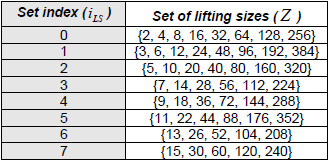
NOTE : This table can be generated by the rule : base_Z x 2^j , where base_Z = the first elements in the set, j = [0 7]
|
Set index (iLS) |
base_Z |
Set of lifting sizes (Z) |
|---|---|---|
|
0 |
2 |
{2 · 20 = 2, 2 · 21 = 4, 2 · 22 = 8, 2 · 23 = 16, 2 · 24 = 32, 2 · 25 = 64, 2 · 26 = 128, 2 · 27 = 256} |
|
1 |
3 |
{3 · 20 = 3, 3 · 21 = 6, 3 · 22 = 12, 3 · 23 = 24, 3 · 24 = 48, 3 · 25 = 96, 3 · 26 = 192, 3 · 27 = 384} |
|
2 |
5 |
{5 · 20 = 5, 5 · 21 = 10, 5 · 22 = 20, 5 · 23 = 40, 5 · 24 = 80, 5 · 25 = 160, 5 · 26 = 320, 5 · 27 = 640} |
|
3 |
7 |
{7 · 20 = 7, 7 · 21 = 14, 7 · 22 = 28, 7 · 23 = 56, 7 · 24 = 112, 7 · 25 = 224, 7 · 26 = 448, 7 · 27 = 896} |
|
4 |
9 |
{9 · 20 = 9, 9 · 21 = 18, 9 · 22 = 36, 9 · 23 = 72, 9 · 24 = 144, 9 · 25 = 288, 9 · 26 = 576, 9 · 27 = 1152} |
|
5 |
11 |
{11 · 20 = 11, 11 · 21 = 22, 11 · 22 = 44, 11 · 23 = 88, 11 · 24 = 176, 11 · 25 = 352, 11 · 26 = 704, 11 · 27 = 1408} |
|
6 |
13 |
{13 · 20 = 13, 13 · 21 = 26, 13 · 22 = 52, 13 · 23 = 104, 13 · 24 = 208, 13 · 25 = 416, 13 · 26 = 832, 13 · 27 = 1664} |
|
7 |
15 |
{15 · 20 = 15, 15 · 21 = 30, 15 · 22 = 60, 15 · 23 = 120, 15 · 24 = 240, 15 · 25 = 480, 15 · 26 = 960, 15 · 27 = 1920} |
In the 3GPP TS 38.212 standard, the lifting sizes are capped at 384. The table above follows the mathematical "doubling" rule strictly, but in practical 5G implementation, values exceeding 384 are typically not used for these specific sets.
Removing the capped number, we can the following table which is same as 38.212 - Table 5.3.2-1
|
Set index (iLS) |
base_Z |
Set of lifting sizes (Z) |
|---|---|---|
|
0 |
2 |
{2, 4, 8, 16, 32, 64, 128, 256} |
|
1 |
3 |
{3, 6, 12, 24, 48, 96, 192, 384} |
|
2 |
5 |
{5, 10, 20, 40, 80, 160, 320} |
|
3 |
7 |
{7, 14, 28, 56, 112, 224} |
|
4 |
9 |
{9, 18, 36, 72, 144, 288} |
|
5 |
11 |
{11, 22, 44, 88, 176, 352} |
|
6 |
13 |
{13, 26, 52, 104, 208} |
|
7 |
15 |
{15, 30, 60, 120, 240} |
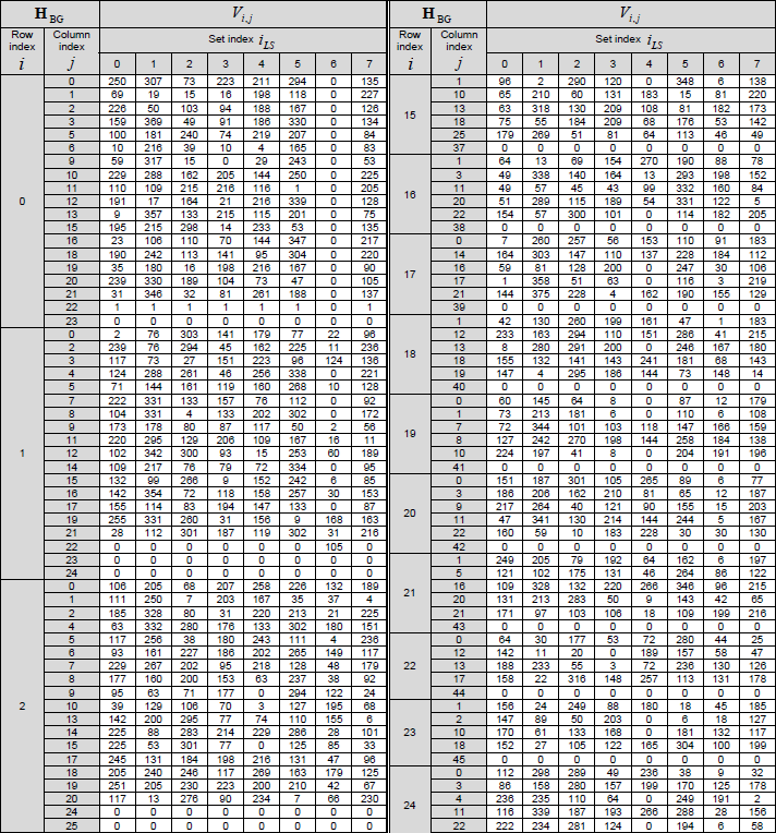
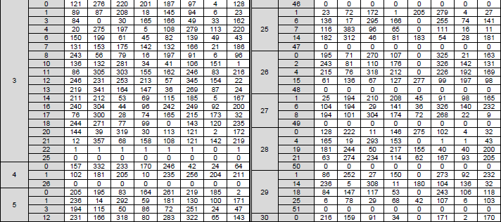
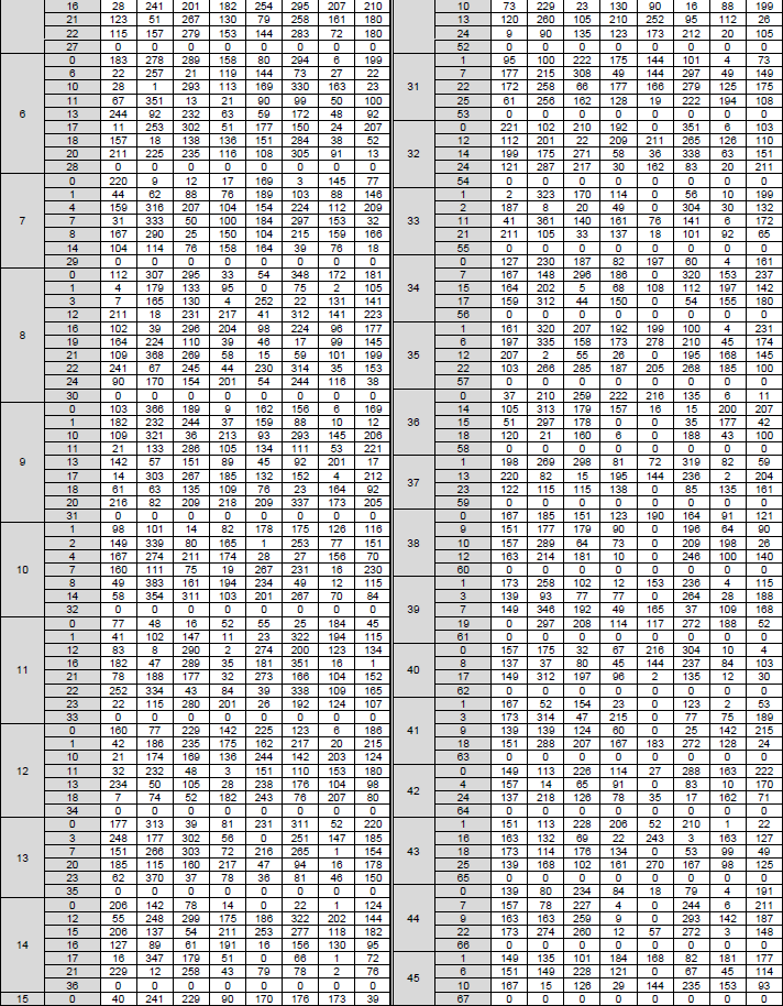
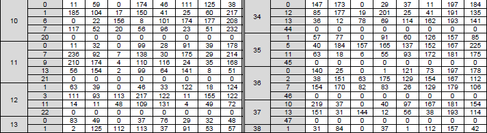
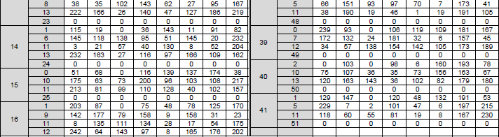
< 38.212-Table 5.3.2-2: LDPC base graph 1 (HBG) and its parity check matrices ( Vi,j) >
The structure, role of this table can be described as below :
- Purpose: This table defines the structure of LDPC Base Graph 1 and the associated shift values Vi,j.
- Structure:
- Base Graph 1 (HBG): A binary matrix with 46 rows (check nodes) and 68 columns (variable nodes). The first 22 columns correspond to information bits, and the remaining columns correspond to parity bits.
- Elements: The table specifies the positions (i, j) where HBG has a value of 1 (indicating a connection between a check node i and a variable node j). All other positions are 0.
- Shift Values (Vi,j): For each position (i, j) where HBG is 1, the table provides a shift value Vi,j. This value depends on the set index iLS (from Table 5.3.2-1) and is used to define the circular permutation matrix that replaces the 1 in the lifted matrix H.
- Role in LDPC: Base Graph 1 is used when the code block length K ≤ 8448. The shift values Vi,j are used to construct the parity-check matrix H by determining the cyclic shifts in the submatrices.
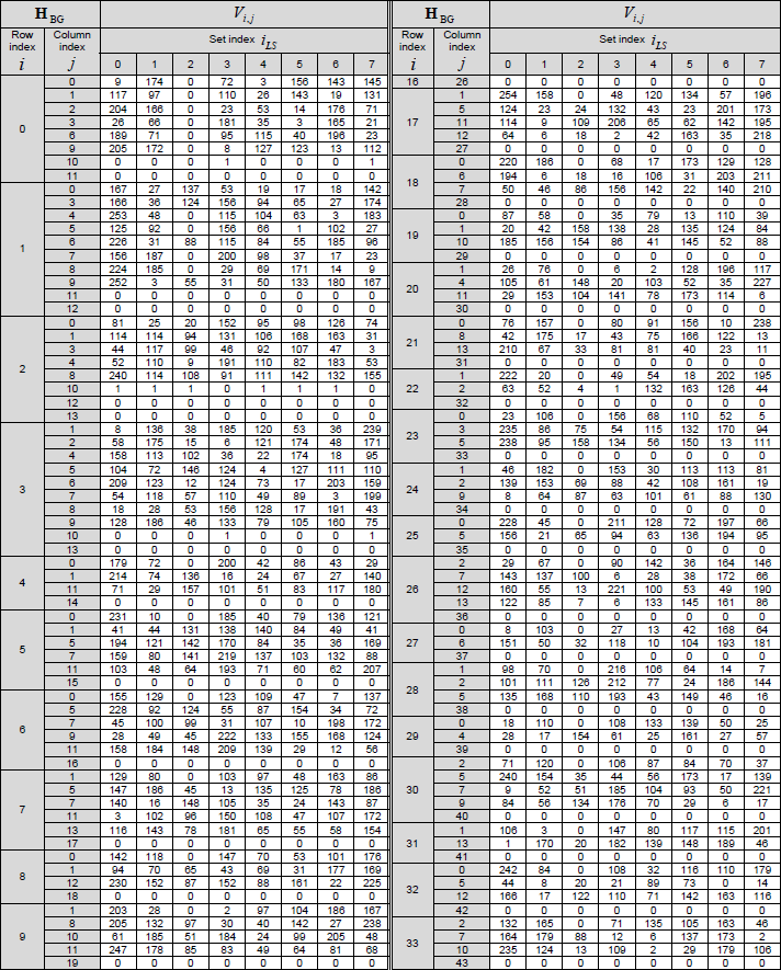
< 38.212-Table 5.3.2-3: LDPC base graph 2 (HBG) and its parity check matrices ( Vi,j) >
The structure, role of this table can be described as below :
Table 5.3.2-3: LDPC Base Graph 2 (HBG) and its Parity Check Matrices (Vi,j)
- Purpose: This table defines the structure of LDPC Base Graph 2 and the associated shift values Vi,j.
- Structure:
- Base Graph 2 (HBG): A binary matrix with 42 rows (check nodes) and 52 columns (variable nodes). The first 22 columns correspond to information bits, and the remaining columns correspond to parity bits.
- Elements: Similar to Table 5.3.2-2, this table specifies the positions (i, j) where HBG has a value of 1, with all other positions being 0.
- Shift Values (Vi,j): For each position (i, j) where HBG is 1, the table provides a shift value Vi,j, which also depends on the set index iLS.
- Role in LDPC: Base Graph 2 is used when the code block length K > 8448. The shift values Vi,j serve the same purpose as in Table 5.3.2-2, defining the cyclic shifts for the lifted matrix H.
LDPC Encoding
At first, I tended to think of encoding as the less mysterious half of LDPC. The transmitter already knows the data, so it seemed that the encoder only had to add some parity bits and send the result. Compared with decoding, where the receiver has to struggle with noise and uncertainty, encoding looked almost too straightforward.
But once I looked more carefully at NR LDPC, I realized that encoding also has its own structure. The encoder does not begin by writing one giant H matrix and blindly solving everything from there. It first decides how the transport block should be prepared, which base graph should be used, how large the lifted structure must become, where filler bits are needed, and how many coded bits can actually be transmitted over the available radio resource.
So the key realization was this:
- LDPC encoding is not only about creating parity bits.
- It is also about shaping the information block into the exact NR LDPC structure required for transmission.
- The encoder constructs a codeword that satisfies H c = 0.
- Then rate matching and modulation reshape that protected codeword into the exact bit stream and symbols that can be sent over the air.
Following is the overall flow of LDPC encoding in the order used by a real transmitter.
- Step 1 : Receive the transport block from higher layer
- Step 2 : Attach the transport-block CRC
- Step 3 : Segment the block if it is too large
- Step 4 : Attach code-block CRC when segmentation is used
- Step 5 : Select the proper NR LDPC base graph
- Step 6 : Determine the lifting size Zc
- Step 7 : Insert filler bits if the LDPC input is larger than the real information block
- Step 8 : Construct or identify the parity-check structure H
- Step 9 : Place the information bits into the systematic part of the codeword
- Step 10 : Generate parity bits so that H c = 0
- Step 11 : Form the LDPC code block
- Step 12 : Puncture the first 2 Zc bits of the mother code
- Step 13 : Select bits from the circular buffer according to redundancy version
- Step 14 : Repeat or omit bits to match the available radio resource
- Step 15 : Interleave the selected coded bits
- Step 16 : Scramble the coded bit stream
- Step 17 : Map bits to modulation symbols
- Step 18 : Transmit the encoded symbols over the air
Step 1 : Receive the transport block from higher layer
This is the true starting point of LDPC encoding.
The transmitter does not begin with parity bits, matrices, or lifting sizes. It begins with a transport block from the higher layer. These are the real information bits that eventually have to survive the radio channel.
This is already different from decoding. The receiver begins with uncertainty. The encoder begins with certainty. It already knows exactly what message it wants to protect.
So the first question is very simple, but also very important:
What is the actual information block that must be carried safely through the whole physical-layer process ?
Once that block is known, the next question naturally appears. If the receiver later recovers some bits, how will it know whether they are really correct ?
Conceptually, this is the payload that later becomes `A`, the transport-block size used throughout the NR processing chain.
| A = int(tbs) |
Step 2 : Attach the transport-block CRC
Before the encoder starts adding LDPC parity, it first attaches a CRC to the transport block.
At first, this can feel redundant. LDPC already has parity checks, so why add another check before encoding ? The reason is that the two kinds of checks serve different purposes.
- LDPC parity checks help the decoder repair errors.
- CRC helps the receiver decide whether the final recovered transport block can be trusted.
This distinction matters. A codeword may satisfy the LDPC structure and still not be the originally transmitted message. CRC gives the receiver a final integrity test outside the LDPC graph itself.
So at this stage, the encoder is asking:
How can I attach a small signature to the information block so the receiver can later judge whether the recovered result is truly valid ?
Now the block has become slightly larger. The next question is whether it still fits comfortably into one LDPC code block.
The receiver-side implementation reconstructs the same TB-CRC length from the transport-block size.
| L_tb = 24 if A > 3824 else 16 B = A + L_tb |
Step 3 : Segment the block if it is too large
Now the encoder has a block containing the original information plus the transport-block CRC.
But one LDPC code block cannot be allowed to grow without limit. If the block is too large, the complexity of encoding and decoding would also become too large. So NR asks a practical question before moving further:
Can this whole block be handled as one LDPC code block, or should it be divided into smaller pieces ?
If the block is small enough, it remains as one code block. If it is too large, it is segmented. This keeps the LDPC operation manageable and lets each part be processed with a bounded code-block size.
So segmentation is not mainly about changing the information. It is about fitting the information into a structure that the LDPC machinery can handle efficiently.
But once the block is split into several pieces, another question appears. If one piece is decoded incorrectly later, how will the receiver know which piece failed ?
The current Python receiver computes the same segmentation parameters that an encoder would have used.
| if B <= K_cb: C = 1 L_cb = 0 else: C = int(np.ceil(B / (K_cb - 24))) L_cb = 24 |
Step 4 : Attach code-block CRC when segmentation is used
If segmentation produced more than one code block, each code block receives its own CRC.
This is easy to overlook because the transport block already had a CRC. But after segmentation, each code block becomes a separate unit for LDPC processing. If one of them fails while the others succeed, the receiver benefits from knowing that at the code-block level.
So the encoder adds a local check to each segmented block. This gives the receiver two levels of confidence later:
- a code-block level check for each decoded piece, and
- a transport-block level check after the pieces are combined again.
The question at this stage is:
If the transport block has been split apart, how can each piece carry enough self-checking information to be verified on its own ?
Now the information has been prepared. The next question is no longer about CRC. It is about which LDPC structure should carry this block.
In the receiver, the corresponding code-block CRC is checked only when more than one code block exists.
| if seg['C'] > 1: computed, received, _, _ = _crc_check_generic( info_bits, poly=0x1864CFB, order=24 ) |
Step 5 : Select the proper NR LDPC base graph
Now the encoder has to choose the LDPC family itself.
NR does not use one single fixed LDPC matrix for every situation. Instead, it provides two standard base graphs. One is better suited to larger blocks and higher code rates. The other is better suited to smaller blocks or lower code rates.
This is one of the most important NR-specific decisions. The encoder is not yet constructing the full H matrix. It is first choosing the small structural template from which the final matrix will later be created.
So the encoder asks:
Given this block size and this operating point, which standard LDPC skeleton should I start from ?
Once the base graph is chosen, the rough shape of the code is known. But it is still only a small template. The next question is: how large should that template become ?
The decoder repeats the same selection rule so both sides agree on the LDPC structure.
| if A <= 292 or (A <= 3824 and r <= 0.67) or r <= 0.25: bg = 2 else: bg = 1 |
Step 6 : Determine the lifting size Zc
The selected base graph is still too small to encode a real code block directly.
It is more like a blueprint than a finished building. The lifting size Zc tells the encoder how much that blueprint should be expanded. Every valid base-graph entry becomes a Zc by Zc block, and the final LDPC structure scales with that choice.
The encoder cannot choose any arbitrary value. NR defines a set of allowed lifting sizes, and the encoder must select one large enough to hold the required information bits.
So the question becomes:
How large must the LDPC structure become so that this code block fits, while still using one of the allowed standardized lifting sizes ?
After this choice, the encoder knows the required LDPC input size. But sometimes the real information block is still slightly smaller than that size. Then one more adjustment is needed.
The Python receiver recovers the same lifting size from the same allowed set.
| Z_candidates = [z for z in ALL_Z_VALUES if K_b * z >= K_prime] Z_c = min(Z_candidates) |
Step 7 : Insert filler bits if the LDPC input is larger than the real information block
Once the LDPC input size is fixed, the encoder may discover a small mismatch.
The chosen structure may have room for more information positions than the real code block actually needs. The encoder cannot leave those positions undefined. So it inserts filler bits into the unused positions, usually known zeros.
These filler bits are not user data. They are more like temporary placeholders that let the real information fit neatly into the rigid LDPC input shape selected by the standard.
This step answers the question:
If the standard LDPC input structure is slightly larger than my real information block, what should occupy the unused positions ?
Now every required information-side position has a defined value. The next question is about the rule that the entire future codeword must obey.
The receiver later identifies these same filler locations and treats them as known zeros.
| F = K - K_prime filler_positions = range(K_prime, K) |
Step 8 : Construct or identify the parity-check structure H
With the base graph and lifting size fixed, the encoder now knows the parity-check structure H that defines the code.
This is a subtle but important shift. Until now, the encoder was preparing the information block. From this point onward, it starts preparing the mathematical rule that the full codeword must satisfy.
In practice, NR does not need to store one huge dense matrix. The quasi-cyclic structure lets the implementation describe H compactly from the base graph, shift values, and lifting size. But conceptually, the meaning is the same: H tells which bit positions participate in which parity equations.
So the encoder is now asking:
What exact parity-check structure must the final codeword satisfy ?
Once H is known, there is still a practical question left. Where do the original information bits go inside the codeword that must satisfy H c = 0 ?
The receiver-side implementation reconstructs the same graph structure from the NR parameters.
| check_edges, var_edges, edge_vars = _build_ldpc_graph( 'bg2', z_c, int(i_ls) ) |
Inside this function, the implementation first loads the selected base-graph table for the chosen lifting-set index. Then it walks through every base-graph row and column. A value smaller than 0 means there is no connection at that location. A valid shift value means that one base-graph entry must become a whole shifted circulant pattern after lifting.
So the code does not build one giant dense H matrix cell by cell. Instead, it directly creates the graph connections that the decoder will need later.
- check_edges tells which edges belong to each lifted check node.
- edge_vars tells which variable node is connected to each edge.
- var_edges is then built in the reverse direction, telling which edges touch each variable node.
In other words, the quasi-cyclic matrix description is converted directly into a Tanner-graph representation.
| bm = _load_bg2(int(i_ls)) check_edges = [] edge_vars = [] for bg_row in range(bm.shape[0]): row_edges = [[] for _ in range(z_c)] for bg_col in range(bm.shape[1]): shift = int(bm[bg_row, bg_col]) if shift < 0: continue for local_row in range(z_c): var = bg_col * z_c + ((local_row + shift) % z_c) edge_vars.append(var) row_edges[local_row].append(len(edge_vars) - 1) check_edges.extend(row_edges) |
After that first pass, the implementation builds the reverse lookup for variable nodes:
| var_edges = [[] for _ in range(bm.shape[1] * z_c)] for edge_idx, var_idx in enumerate(edge_vars): var_edges[int(var_idx)].append(edge_idx) |
This is also where the standard table becomes real code.
The values from 38.212 Table 5.3.2-3, the LDPC Base Graph 2 table, are stored in the project as a machine-readable file:
| pylib/vendor/ldpc_codes/5G_bg2.csv |
The implementation does not copy the whole 3GPP table directly into the Python source file. Instead, `_load_bg2(i_ls)` reads this CSV file and rebuilds the BG2 matrix for the selected lifting-set index.
| def _load_bg2(i_ls): path = Path(__file__).resolve().parent / 'vendor' / 'ldpc_codes' / '5G_bg2.csv' bm = np.full((_BG2_ROWS, _BG2_COLS), -1, dtype=np.int16) ... bm[row_idx, col_idx] = int(float(fields[i_ls + 2])) return bm |
The meaning of this is very direct.
- The row index and column index come from the Base Graph 2 position (i, j).
- The selected column `fields[i_ls + 2]` gives the corresponding shift value Vi,j for the chosen lifting-set index.
- If a position has no valid connection, it remains `-1`.
- If a position has a valid shift value, that number is later used by `_build_ldpc_graph()` to create the lifted circular connection pattern.
So the flow is:
- 3GPP Table 5.3.2-3 defines the BG2 positions and shift values.
- `5G_bg2.csv` stores those values in a convenient form for the program.
- `_load_bg2(i_ls)` selects the proper Vi,j value set.
- `_build_ldpc_graph()` expands those values into the actual lifted Tanner-graph connections used by the decoder.
This is a very important point. The standard table is not only a reference table for documentation. In a real implementation, it is the compact description from which the actual LDPC graph is reconstructed.
Step 9 : Place the information bits into the systematic part of the codeword
NR LDPC is systematic. That means the original information bits are placed directly into designated positions of the codeword rather than being hidden inside a completely transformed representation.
This is helpful because it gives the codeword a clear division:
- one part carries the information side, and
- the remaining part will be filled with parity bits chosen to satisfy the LDPC equations.
The filler bits, if any, occupy part of the systematic side as known placeholders. The true payload bits remain distinguishable from them.
So at this stage, the encoder asks:
Which positions of the future codeword should contain the original information, before I solve for the parity part ?
Now the known part of the codeword is placed. The unknown part is the parity portion. This leads directly to the heart of encoding.
The decoder later takes the first information positions back out after decoding.
| codeword[:K_prime] = info_bits codeword[K_prime:K] = filler_bits |
Step 10 : Generate parity bits so that H c = 0
This is the point where LDPC encoding truly earns its name.
The encoder already knows the information bits and the parity-check structure. What remains is to choose parity bits so that the complete codeword satisfies:
H c = 0
Unlike decoding, there is no uncertainty here. The encoder is not guessing which codeword was sent. It is deliberately constructing one valid codeword from known information bits.
The conceptual question is:
Given the information bits already fixed in the systematic positions, what parity bits must be chosen so that every LDPC parity equation is satisfied ?
Once those parity bits are found, the codeword is mathematically valid. But the encoder is not finished, because a valid mother codeword is not always the exact sequence that will be transmitted over the radio.
The current project is receiver-side, so it does not contain a production LDPC encoder. This small fragment shows the condition the encoder must satisfy.
| # choose parity_bits so that # H @ codeword.T == 0 (mod 2) codeword = np.concatenate([systematic_bits, parity_bits]) |
Step 11 : Form the LDPC code block
After the parity bits are generated, the encoder now has a complete LDPC code block.
This is an important milestone. Earlier steps prepared information, selected structure, and solved parity constraints. Now all of those decisions have become one concrete codeword that satisfies H c = 0.
The code block contains:
- systematic information positions,
- possible filler positions, and
- parity positions.
At first, it may seem that this code block should simply be transmitted as it is. But NR still has one more reality to deal with: the radio resource may not have room, or may not need, every bit of the mother codeword.
So the next question is:
Which parts of this valid mother codeword are actually prepared for transmission ?
The receiver later refers to the corresponding lengths as K and N.
| K = 22 * Z_c if bg == 1 else 10 * Z_c N = 66 * Z_c if bg == 1 else 50 * Z_c |
Step 12 : Puncture the first 2 Zc bits of the mother code
In NR LDPC, the transmitted stream does not begin by sending every bit of the mother codeword.
The first 2·Zc bits are punctured. In other words, they belong to the underlying mother-code structure but are not transmitted over the air. The receiver later knows that these positions existed even though no direct channel observation was received for them.
This is one of those details that makes NR LDPC feel less like a textbook block code and more like a practical radio system. The code structure and the transmitted sequence are related, but not identical.
So the encoder asks:
Which mother-code positions are structurally present, but intentionally not sent as part of the transmitted bit stream ?
After puncturing, the encoder still may have more coded bits than the resource allocation can carry. Now it needs a controlled way to choose which coded bits will go out in this transmission.
The decoder mirrors this by inserting neutral LLRs at those punctured positions before belief propagation.
| mother_codeword = full_codeword transmitted_buffer = mother_codeword[2 * Z_c:] |
Step 13 : Select bits from the circular buffer according to redundancy version
The encoder now enters the circular-buffer view of rate matching.
The coded bits are treated as positions in a circular buffer. Depending on the redundancy version, the encoder begins reading from a different starting point. This is how different HARQ transmissions can emphasize different portions of the same underlying codeword.
This is not random selection. It is a standardized pattern that gives the receiver a predictable way to combine information across transmissions later.
The question at this point is:
From which position in the circular buffer should this particular transmission begin selecting coded bits ?
Once the starting point is known, one more practical constraint remains: exactly how many coded bits are needed for the scheduled radio resource ?
The receiver computes the same starting point `k0` when reversing rate matching.
| k0 = compute_k0(rv=rv_idx, bg=bg, Z_c=Z_c, N_cb=N_cb) selected_bits = circular_buffer_read(buf, start=k0, length=E) |
Step 14 : Repeat or omit bits to match the available radio resource
The available physical resource determines the target number of coded bits that can be transmitted.
If fewer bits are needed than the mother structure contains, some bits are not selected in this transmission. If more bits are needed, the circular buffer may wrap and some coded bits may be repeated. This is the reason the word rate matching is so appropriate. The encoder is matching the coded output to the actual resource situation.
So the encoder asks:
How do I reshape the protected LDPC output so that its length exactly matches the number of coded bits the radio allocation can carry ?
Now the right number of bits has been chosen. But before mapping them into modulation symbols, NR still rearranges their order in a specific way.
The receiver computes `E` for each code block and later rebuilds the buffer from that number of received bits.
| E_per_cb = compute_E_per_cb(G=G, C=C, Q_m=Q_m, layers=layers) |
Step 15 : Interleave the selected coded bits
The selected coded bits are now interleaved.
Interleaving can look like a simple shuffling step, but it has a purpose. It arranges the bit stream so that the different bit positions within a modulation symbol receive coded bits in the NR-defined order. This makes the later modulation mapping compatible with the transmission format expected by the receiver.
It is useful to think of this as another alignment step. Earlier, the encoder aligned the information with the LDPC structure. Now it aligns the coded output with the modulation structure.
The key question becomes:
Before I group bits into symbols, in what order should the selected coded bits be arranged ?
After the order is settled, the bits are still too regular to transmit directly. The encoder next applies scrambling.
The receiver later undoes this interleaving before LDPC decoding.
| for i in range(Q_m): for j in range(cols): f[Q_m * j + i] = e[i * cols + j] |
Step 16 : Scramble the coded bit stream
Now the encoder scrambles the coded bit stream.
Scrambling does not replace LDPC coding, and it is not a second error-correcting code. Its role is different. It prevents undesirable long patterns, helps randomize the transmitted sequence, and ties the transmission to parameters such as the RNTI and cell identity.
This is another good example of how the physical layer combines several kinds of processing that serve different purposes:
- LDPC gives error-correction structure.
- Rate matching gives resource adaptation.
- Scrambling gives sequence randomization and transmission-specific identity.
The encoder is now asking:
How can I make the transmitted coded sequence less pattern-prone while keeping it perfectly reversible at the receiver ?
After scrambling, the data is finally ready to leave the bit domain and become constellation symbols.
The receiver reverses this by sign-flipping LLRs with the same Gold sequence.
| c_init = pdsch_c_init(n_rnti, q, n_cell_id) scrambled_bits = bits ^ generate_gold_sequence(len(bits), c_init) |
Step 17 : Map bits to modulation symbols
Only now does the encoder perform modulation mapping.
Several bits are grouped together and mapped onto one complex-valued constellation point. With QPSK, each symbol carries two bits. With 16QAM, each symbol carries four bits. With 64QAM, each symbol carries six bits.
This is an important transition. Up to this point, the encoder has been working with abstract binary sequences. After this step, the protected information becomes actual transmit symbols that will occupy the radio resource grid.
So the question changes form:
How should this final coded bit stream be represented as physical symbols that the transmitter can place onto the air interface ?
Once symbols exist, the encoder-side construction is essentially complete. The next step is no longer about creating more structure. It is about sending the result into the channel.
For the present SIB1 path, the receiver uses a QPSK demapper because SIB1 decoding here is QPSK-based.
| # QPSK example symbol = ((1 - 2*b0) + 1j*(1 - 2*b1)) / np.sqrt(2) |
Step 18 : Transmit the encoded symbols over the air
At the end of encoding, the transport block has gone through a long transformation.
- It received CRC protection.
- It was fitted into one or more LDPC code blocks.
- It was given parity bits so that H c = 0.
- It was rate matched, interleaved, scrambled, and modulated.
The transmitter has now finished the construction process. What leaves the transmitter is no longer just the original information block. It is a carefully prepared waveform designed to survive the wireless channel.
This naturally leads to the final encoding-side question:
Now that the codeword has been constructed and mapped into symbols, what happens when the channel begins to distort it ?
That is exactly where the next section begins. Encoding ends with a deliberately constructed signal. Decoding begins with an uncertain observation of that signal after the real world has had its effect on it.
The decoder begins later from the equalized received symbols `eq_data` rather than from the original clean bits.
| llrs_raw = qpsk_soft_demap(eq_data, n0=n0) |
LDPC Decoding
At first, I thought LDPC decoding would be a simple reverse process of LDPC encoding. In many technologies, this kind of thinking works reasonably well. If the transmitter performs a certain sequence of operations, the receiver often performs the reverse sequence to recover the original data. So I naturally expected LDPC decoding to work in the same way. The encoder creates parity bits from information bits, so I thought the decoder would somehow reverse that operation and directly recover the original information bits.
But LDPC decoding does not really work that way. The receiver does not receive a clean encoded bit sequence. It receives noisy, uncertain channel observations. Because of this, decoding cannot be just an inverse calculation. The decoder has to make a best guess from unreliable evidence. It knows the LDPC structure, but it does not know which received bits are correct and which ones are wrong.
This is where LDPC decoding becomes interesting. Instead of reversing the encoder step by step, the decoder uses the parity check matrix H as a rule book. It asks whether the current candidate codeword satisfies H c = 0. If not, it does not simply flip bits one by one. It lets variable nodes and check nodes exchange soft messages through the Tanner graph. Each iteration refines the belief about every bit by combining the channel evidence and the parity constraints.
So the key realization was this:
- LDPC encoding is a construction process.
- LDPC decoding is an inference process.
- The encoder constructs a valid codeword.
- The decoder tries to infer the most likely valid codeword from noisy observations.
If the parity checks pass, the LDPC part looks successful. But the final trust comes from CRC. If CRC passes, the decoded transport block is delivered. If not, HARQ gives the receiver another chance by combining more soft information from retransmission.
So the real beauty of LDPC decoding is not just in the matrix or the graph. It is in the way uncertain channel evidence and strict parity structure keep interacting until the receiver either finds a consistent message or admits that it needs more evidence.
Following is the overall flow of LDPC decoding in the order used by a real receiver.
- Step 1 : Receive the noisy channel symbols
- Step 2 : Demodulate the received symbols
- Step 3 : Calculate soft values for each coded bit
- Step 4 : Generate LLR values for all received bits
- Step 5 : Select the proper NR LDPC base graph
- Step 6 : Determine the lifting size Zc
- Step 7 : Undo bit interleaving if applied
- Step 8 : Remove rate-matching effects before LDPC decoding
- Step 9 : Place known filler-bit values into the decoder input if needed
- Step 10 : Construct or identify the parity check matrix H
- Step 11 : Build the Tanner graph from H
- Step 12 : Initialize variable nodes with the prepared LLR values
- Step 13 : Initialize check node messages
- Step 14 : Start iterative message passing
- Step 15 : Send messages from variable nodes to check nodes
- Step 16 : Update messages at check nodes using parity check constraints
- Step 17 : Send updated messages from check nodes back to variable nodes
- Step 18 : Update variable node beliefs using channel LLR and incoming check node messages
- Step 19 : Make tentative hard decisions for all bits
- Step 20 : Check whether the tentative codeword satisfies H c = 0
- Step 21 : If all parity checks pass, stop decoding
- Step 22 : If parity checks fail, continue to the next iteration
- Step 23 : Repeat message passing until success or maximum iteration count is reached
- Step 24 : If decoding succeeds, extract the systematic information bits
- Step 25 : Remove filler bits from the decoded information block if used
- Step 26 : Perform CRC check
- Step 27 : If CRC passes, deliver the decoded transport block
- Step 28 : If CRC fails, declare decoding failure or request retransmission through HARQ
Step 1 : Receive the noisy channel symbols
This is the very first input to the LDPC decoding process.
At the transmitter side, the original transport block is encoded by LDPC. Then the encoded bits are rate matched, scrambled, modulated, and transmitted over the air.
But the receiver does not receive clean bits.
The receiver receives radio signals that have passed through the wireless channel.
So the received signal may be distorted by many things.
- Noise is added.
- Fading changes the amplitude and phase.
- Interference may be mixed in.
- The channel may rotate the constellation points.
- The receiver may also have some timing or frequency error.
So at this point, the receiver is not seeing something like this:
0 1 1 0 1 0 0 1
Instead, it receives complex-valued symbols.
For example, in QPSK, the transmitter may send one constellation point representing two bits. But at the receiver, that point may not appear exactly at the ideal position. It may be shifted, rotated, or blurred.
So the receiver may see something like this:
0.72 + j0.65
-0.81 + j0.54
0.12 - j0.95
-0.40 - j0.30
These are not bits yet.They are noisy channel symbols. This is an important point.
LDPC decoding does not start from perfect 0 and 1 values. It starts from uncertain information.
The receiver first has to ask:
- How likely is this received symbol to represent bit 0 ?
- How likely is it to represent bit 1 ?
- How confident am I about that decision ?
- This uncertainty is very important for LDPC decoding.
If the receiver immediately converts every received symbol into hard bits, a lot of useful information is lost. For example, a received symbol very close to the ideal 0 position and another symbol barely on the 0 side would both become 0. But their reliability is very different.
LDPC decoding needs this reliability information.
So in this first step, the receiver simply collects the noisy received symbols from the channel. These symbols are still analog-like or complex-valued digital samples after RF/baseband processing. They are not yet the final decoded bits.
The main question at this stage is:
What did the channel give us, and how uncertain is it ?
In the Python implementation, this input is the equalized PDSCH symbol stream passed into the SIB1 decoder. At this point, the values are still complex-valued channel observations, not decoded bits.
| def decode_sib1_pdsch(eq_data, mcs, rv_idx, n_prb, ...): result = {'steps': {}, 'error': None} llrs_raw = qpsk_soft_demap(eq_data, n0=n0) |
Step 2 : Demodulate the received symbols
After the receiver gets the noisy channel symbols, the next step is demodulation. The received symbols are still complex values. They are not bits yet.
For example, in QPSK, each transmitted symbol represents 2 bits. In 16QAM, each symbol represents 4 bits. In 64QAM, each symbol represents 6 bits. In 256QAM, each symbol represents 8 bits.
So the receiver has to map each received constellation point back to the possible bit values. But there is an important point here.
The receiver should not simply say:
- This symbol is 00.
- This symbol is 01.
- This symbol is 10.
- This symbol is 11.
That would be hard demodulation.
For LDPC decoding, this is usually not enough. Instead, the receiver tries to estimate how likely each bit is to be 0 or 1.
For example, assume QPSK.
If the received point is very close to the ideal constellation point for 00, then the receiver can be highly confident that the bits are 00.
But if the received point is near the boundary between 00 and 01, the receiver should not be too confident. It may say:
- The first bit is probably 0.
- The second bit is uncertain.
This is the key idea of soft demodulation. The demodulator does not just produce decoded bits. It produces reliability information for each bit. This reliability information later becomes LLR values.
So demodulation is the bridge between the noisy constellation symbols and the LDPC decoder.
The channel gives us distorted symbols.
The demodulator converts those symbols into bit-level confidence.
At this stage, the receiver is not yet correcting errors. It is only preparing useful soft information for the LDPC decoder.
The important question here is:
For each received symbol, how strongly does it suggest each bit is 0 or 1 ?
In the implementation, demodulation is performed by the QPSK soft demapper. It converts each complex symbol into two bit-level soft values rather than making only a hard 0 or 1 decision.
| def qpsk_soft_demap(eq_data, n0=1.0): eq = np.asarray(eq_data).reshape(-1) out = np.empty(2 * eq.size, dtype=np.float32) |
Step 3 : Calculate soft values for each coded bit
After demodulation, the receiver does not want to produce only hard bit values like 0 or 1.
It wants to produce soft values.
A soft value means:
- How likely is this coded bit to be 0 ?
- How likely is this coded bit to be 1 ?
How confident is the receiver about this judgment ?
This is very important for LDPC.
LDPC decoding works much better when it knows not only the estimated bit value, but also the reliability of that bit.
For example, assume the receiver has two received bits.
- The first one looks very clearly like 0.
- The second one looks only slightly more like 0 than 1.
If we use hard decision, both become 0.
But from the LDPC decoder point of view, these two bits are very different.
- The first bit is a strong 0.
- The second bit is a weak 0.
This difference matters a lot.
During LDPC decoding, the decoder may decide that the weak 0 should actually be flipped to 1 if the parity check constraints suggest so. But it will be more reluctant to change the strong 0 because the channel observation was more confident.
So the soft value is like the first opinion from the channel.
It does not say:
- This bit is definitely 0.
It says something more like:
- This bit seems to be 0, and I am quite confident. , or:
- This bit seems to be 0, but I am not very sure. or:
- This bit seems to be 1, and I am strongly confident.
In practical systems, this soft value is usually represented as an LLR, Log-Likelihood Ratio.
But before going into the exact LLR formula, the important idea is simple.
The receiver assigns a reliability value to every coded bit.
This means every bit entering the LDPC decoder carries two kinds of information.
- One is the preferred bit direction.
- The other is the confidence level.
So this step is not yet LDPC decoding itself.
It is preparation for LDPC decoding.
The main question at this stage is:
For each coded bit, how much should the decoder trust the channel observation ?
The soft values are formed from the real and imaginary parts of each QPSK symbol. Their sign tells the likely bit direction, and their magnitude carries the confidence.
| scale = float(np.sqrt(2) / max(n0 / 2.0, 1e-6)) out[0::2] = -np.real(eq).astype(np.float32) * scale out[1::2] = -np.imag(eq).astype(np.float32) * scale |
The current SIB1 implementation only needs QPSK. If the same receiver were extended to higher-order modulation such as 16QAM or 64QAM, the demapper would no longer produce only two LLRs from the real and imaginary axes. It would evaluate every constellation point and generate one LLR for each bit position carried by the symbol.
| def qam_soft_demap(eq, constellation, bit_labels, n0): n_bits = bit_labels.shape[1] llrs = np.empty((len(eq), n_bits), dtype=np.float32) for k in range(n_bits): d0 = np.min(np.abs(eq[:, None] - constellation[bit_labels[:, k] == 0]) ** 2, axis=1) d1 = np.min(np.abs(eq[:, None] - constellation[bit_labels[:, k] == 1]) ** 2, axis=1) llrs[:, k] = (d0 - d1) / max(n0, 1e-6) return llrs.reshape(-1) |
Step 4 : Generate LLR values for all received bits
Now the receiver converts the soft information into a more formal value.
This value is called LLR. LLR means Log-Likelihood Ratio.
The basic idea is simple.
For each received coded bit, the receiver asks:
- Is this bit more likely to be 0 ?
- Or is this bit more likely to be 1 ?
- And how strong is that belief ?
So LLR is not just a bit value. It is a signed confidence value.
In many common conventions:
- Positive LLR means the bit is more likely to be 0.
- Negative LLR means the bit is more likely to be 1.
- Large magnitude means high confidence.
- Small magnitude means low confidence.
So the following values have different meanings:
- +8 means very likely 0.
- +1 means slightly likely 0.
- 0 means almost unknown.
- -1 means slightly likely 1.
- -8 means very likely 1.
This is why LLR is much more useful than hard bits.
A hard bit can only say 0 or 1.
But LLR can say how strongly the receiver believes that 0 or 1 is correct.
For example, two received bits may both be decided as 0 by hard decision.
But their LLR values may be very different. One may be +9. Another may be +0.3.
To the LDPC decoder, these are not the same. The +9 bit is very reliable. The +0.3 bit is weak and suspicious.
During iterative decoding, the weak bit can be changed more easily if the parity check equations disagree with it. But the strong bit will need much stronger evidence before it is changed.
This is the key point.
- The LLR values become the initial belief of the LDPC decoder. They are attached to the variable nodes of the Tanner graph.
- The Tanner graph tells which bits are connected to which parity checks. The LLR tells how much each bit is trusted at the beginning.
- So at this step, the receiver prepares one LLR value for every received coded bit.
From this point, LDPC decoding can start using both pieces of information:
- The known structure from H.
- The uncertain bit reliability from LLR.
The main question at this stage is:
For every bit, how strongly does the received signal support 0 or 1 ?
The decoder records the LLR stream and even keeps simple diagnostics such as minimum, maximum, and mean absolute LLR so the receiver can inspect the quality of the soft information.
| llrs_raw = qpsk_soft_demap(eq_data, n0=n0) result['steps']['1_qpsk_demap'] = { 'n_llrs': int(len(llrs_raw)), 'llr_min': float(np.min(llrs_raw)), 'llr_max': float(np.max(llrs_raw)), } |
Step 5 : Select the proper NR LDPC base graph
Before constructing the LDPC parity check matrix H, the receiver has to know which base graph is used.
In NR LDPC, there are two base graphs.
- Base Graph 1
- Base Graph 2
This is one of the first NR-specific parts of LDPC.
The receiver does not freely choose any random LDPC matrix. It follows the same rule as the transmitter. Based on the transport block size and code rate, both transmitter and receiver select the same base graph.
In simple terms:
- Base Graph 1 is mainly for larger transport blocks and higher code rates.
- Base Graph 2 is mainly for smaller transport blocks or lower code rates.
This matters because the base graph is the seed structure of the whole LDPC matrix.
At this point, the receiver is not yet building the full H matrix.
It first asks:
- Which basic LDPC structure should I start from ?
In NR, this decision is made from parameters such as:
Transport block size
- Code rate
- Number of coded bits
- Modulation and resource allocation related information
A simplified rule is like this:
- Use Base Graph 2 when the block is small or the code rate is low.
- Use Base Graph 1 for larger blocks and relatively higher code rates.
More specifically, NR commonly selects Base Graph 2 when the transport block is very small, or when the transport block is not large and the code rate is not high, or when the code rate is very low. Otherwise, Base Graph 1 is used.
This step is important because everything after this depends on the selected base graph.
- The lifting size depends on it.
- The shift values depend on it.
- The expanded H matrix depends on it.
- The Tanner graph also depends on it.
So the base graph is like the skeleton of the LDPC code.
But it is not yet the full body.
The full H matrix is created later by expanding this base graph using the lifting size and shift values.
The important question at this stage is:
Before building the huge LDPC matrix, which small standard-defined structure should be used as the starting point ?
The base graph is selected from the transport block size and code rate using the same rule as the transmitter. For SIB1-sized blocks, this commonly leads to Base Graph 2.
| if A <= 292 or (A <= 3824 and r <= 0.67) or r <= 0.25: bg = 2 K_cb = 3840 else: bg = 1 K_cb = 8448 |
Step 6 : Determine the lifting size Zc
After selecting the base graph, the next step is to determine the lifting size.
The lifting size is usually written as Zc. This is one of the most important parameters in NR LDPC.
At first, Zc may look like just another number in the specification. But conceptually, it has a very important role.
The base graph itself is only a small matrix. It is not the final parity check matrix H. Each entry in the base graph must be expanded into a bigger block. The size of that block is Zc by Zc.
So Zc tells how much the base graph should be expanded.
- If Zc is small, the final H matrix becomes smaller.
- If Zc is large, the final H matrix becomes larger.
This is why it is called lifting size. It lifts a small base graph into a large real LDPC matrix.
For example, if one entry in the base graph is valid, it may become a Zc x Zc shifted identity matrix.
If one entry in the base graph is -1, it becomes a Zc x Zc all-zero matrix.
So the base graph defines the rough connection pattern.
Zc defines the scale of expansion.
The receiver determines Zc using the same rule as the transmitter. It is mainly related to the code block size after transport block segmentation and the selected base graph.
The receiver has to choose a Zc large enough to fit the required number of information bits in the LDPC code block.
In NR, Zc is not any arbitrary number.
It must be selected from a predefined set of lifting sizes in the specification. This is why the receiver does not just calculate any convenient value. It selects one allowed Zc value that matches the code block requirement.
This step is important because once Zc is chosen, the real size of the LDPC structure becomes fixed.
- The number of rows in H becomes fixed.
- The number of columns in H becomes fixed.
- The size of every shifted identity block becomes fixed.
- The Tanner graph also becomes fixed.
So at this stage, the receiver is asking:
How large should the base graph be expanded so that it can support this code block ?
This is the role of Zc.
It is the scaling factor that turns the small NR base graph into the actual LDPC parity check structure used for decoding.
After the base graph is known, the implementation chooses the smallest allowed lifting size that can hold the code-block information bits.
| Z_candidates = [z for z in ALL_Z_VALUES if K_b * z >= K_prime] Z_c = min(Z_candidates) i_ls = next(i for i, row in enumerate(LIFTING_SIZE_TABLE) if Z_c in row) |
Step 7 : Undo bit interleaving if applied
Before transmission, the encoded bits may be interleaved. Interleaving means the bit order is rearranged.
At first, this may look like a simple permutation. But the reason is important.
Wireless errors are often not evenly spread. Sometimes a group of nearby symbols may be badly affected by fading, interference, or noise. If the bits are transmitted in the original order, this may create a burst of errors in one part of the codeword. That is not good for decoding.
LDPC decoding usually works better when errors are spread out rather than concentrated in one small region. So the transmitter may interleave the bits before modulation or transmission. It spreads nearby coded bits across different modulation positions or resource locations.
At the receiver side, this rearrangement has to be reversed before LDPC decoding can really begin. The receiver must put the bits back into the order expected by the LDPC structure. This is the role of deinterleaving.
Conceptually, the receiver asks: The transmitter shuffled the coded bits before sending them. How do I put them back into the original LDPC codeword order ?
This matters because the parity check matrix H assumes a specific bit order.
Variable node 0 means one specific coded bit.
Variable node 1 means another specific coded bit.
If the LLR values are attached to the wrong variable nodes, the decoder will check the wrong parity relationships. So deinterleaving is not just cosmetic. It restores the correct mapping between received soft bits and LDPC variable nodes.
The important point is this: LDPC decoding does not only need reliable LLR values. It also needs those LLR values to be placed at the correct bit positions.
So this step makes sure the soft information from the channel is aligned with the structure that the LDPC decoder will use next.
In the real receiver flow, the bit interleaver is undone before LDPC decoding so the LLRs return to the codeword-related order expected by rate recovery.
| def undo_bit_interleaver(llrs, q_m): for i in range(q_m): for j in range(cols): out[i * cols + j] = llrs[q_m * j + i] |
Step 8 : Remove rate-matching effects before LDPC decoding
Before LDPC decoding can begin, the receiver still has to remember one thing.
The bits transmitted over the air may not be exactly the same as the full LDPC encoded bit sequence.
Before transmission, NR performs rate matching. This means the transmitter may select, repeat, or skip some encoded bits so that the number of transmitted bits matches the available radio resources.
The LDPC encoder may create a codeword of a certain size. But the PDSCH or PUSCH allocation may allow only a certain number of coded bits to be transmitted. So the transmitter adjusts the encoded bit stream through rate matching.
At the receiver side, this effect must be handled in the reverse direction. This is often called rate dematching.
The receiver has to reconstruct the proper LDPC decoder input from the received soft bits. Some bits may have been punctured. That means they were not transmitted.
For those bits, the receiver has no real channel observation, so their LLR may be filled with neutral values.
Some bits may have been repeated. In that case, the receiver may combine the repeated soft values.
Some bits may have been selected from a circular buffer. So the receiver has to put the received LLR values back into the correct positions before LDPC decoding.
Conceptually, this step asks: The transmitter changed the encoded bit stream to fit the radio resource. How do I undo that mapping so the LDPC decoder receives the bits in the expected codeword positions ?
This is important because LDPC decoding depends on bit positions. The H matrix assumes that each coded bit is in a specific position.
If the received LLRs are placed in the wrong positions, the parity check equations no longer match the intended code structure. So rate dematching is not just a bit rearrangement. It is the step that restores the connection between the received soft bits and the LDPC codeword structure. Without this step, the decoder may be using correct LLR values, but attached to the wrong variable nodes. And that would make the Tanner graph conversation meaningless.
The implementation then performs rate recovery. It places the received LLRs back into the NR circular buffer, combines repetitions, and skips filler positions.
| buf = np.zeros(n_cb, dtype=np.float32) pos = (k0 + step) % n_cb if filler_lo <= pos < filler_hi: continue buf[pos] += llrs_e[j] |
Step 9 : Place known filler-bit values into the decoder input if needed
There is one more practical detail before iterative decoding starts.
In NR LDPC, the original information block does not always fill the whole LDPC input structure. When the real information bits are not enough, filler bits are inserted during encoding so that the block fits the required LDPC size.
These filler bits are not unknown user data. They are known positions, usually treated as zero. So at the receiver side, they should not be treated like ordinary received bits with ordinary uncertainty.
Instead, once the receiver knows the code block structure, it can place very strong known values at the filler positions before LDPC decoding begins.
- The received LLRs carry evidence from the channel.
- The filler positions carry prior knowledge from the code construction itself.
This helps the LDPC decoder because those positions do not need to be guessed in the same way as transmitted bits. They are already known parts of the structure.
So before the Tanner graph conversation starts, the receiver makes sure of one more thing:
Which positions are real received soft bits, and which positions are known filler bits that should already be fixed in the decoder input ?
Known filler positions are not left as unknown received bits. They are clamped to a strong known-zero LLR before the iterative decoder starts.
| buf = np.zeros(N_cb, dtype=np.float32) if flo < fhi: buf[flo:fhi] = -100.0 # known-zero filler LLRs |
Step 10 : Construct or identify the parity check matrix H
After the base graph and lifting size Zc are decided, the receiver can now construct the real parity check matrix H.
This is the matrix used by the LDPC decoder. But in NR, H is usually not stored as one huge matrix full of 0 and 1 values. That would be too large and inefficient. Instead, the receiver constructs H from the standard-defined base graph and lifting size.
The base graph gives the small structure.
- Zc tells how large each block should become.
- Each entry in the base graph is expanded into a Zc x Zc block.
- If the base graph entry is -1, that position becomes an all-zero block.
- If the base graph entry is a valid shift value, that position becomes a circularly shifted identity matrix.
- So one small number in the base graph becomes one whole block in the final H matrix.
This is the key idea.
The final H matrix is not arbitrary. It is a structured matrix.
- It is created by repeating this expansion rule over all entries of the selected base graph.
At this point, the receiver knows the full parity check structure.
- It knows which coded bits participate in which parity checks.
- It knows which variable nodes are connected to which check nodes.
- It knows the rule that a valid codeword must satisfy. It is H c = 0
This does not mean the receiver already knows the correct codeword c. It only means the receiver knows the rule that the correct codeword must satisfy. This is why H is so important.
The LLR values came from the noisy channel. But H comes from the standard-defined LDPC structure.
- One side is uncertain.
- The other side is fixed.
LDPC decoding happens by combining these two.
The receiver asks:
Given these unreliable LLR values from the channel, can I find a codeword that satisfies the fixed parity check matrix H ?
So this step is where the abstract 3GPP tables become the actual decoding structure.
The runtime decoder does not need to store one huge dense matrix. It reconstructs the needed parity-check structure from the standard-defined base graph and lifting parameters.
| check_edges, var_edges, edge_vars = _build_ldpc_graph( 'bg2', z_c, int(i_ls) ) |
Step 11 : Build the Tanner graph from H
After the parity check matrix H is constructed or identified, the same structure can be represented as a graph. This graph is called a Tanner graph.
At first, this may sound like a completely new object. But it is not really new. The Tanner graph is another way of drawing the same information contained in H. The matrix H tells which coded bits are involved in which parity check equations. The Tanner graph shows the same relationship visually.
In the Tanner graph, there are two types of nodes.
- One type is variable node. A variable node represents a coded bit.
- The other type is check node. A check node represents a parity check equation.
Now the question is:
How do we know which variable node is connected to which check node ?
The answer comes directly from H.
- If an entry in H is 1, there is a connection.
- If an entry in H is 0, there is no connection.
For example, if H row 3 column 10 is 1, it means coded bit 10 participates in parity check equation 3. So in the Tanner graph, variable node 10 is connected to check node 3.
This is the important point.
- The Tanner graph is not constructed from the received noisy bits.
- It is not constructed from the LLR values.
- It is not guessed during decoding.
- It is constructed from H.
The received LLR values will be attached to the variable nodes later. But they do not define the graph structure.
So H defines the skeleton. The Tanner graph is the graphical form of that skeleton.
Once this graph is built, LDPC decoding can be understood as message passing on this graph.
- Variable nodes send messages to check nodes.
- Check nodes send messages back to variable nodes.
- These messages are updated again and again.
Through this repeated exchange, each bit gradually receives opinions from the channel and from the parity check constraints.
So this step is where the matrix view changes into a communication view.
- Instead of seeing LDPC as only: H c = 0
- we start seeing it as: Bits and parity checks talking to each other through the connections defined by H.
This is why the Tanner graph is important. It gives a concrete picture of how iterative LDPC decoding happens.
The main question at this stage is:
How can the fixed parity check matrix H be converted into a network of bit nodes and check nodes, so that decoding can be done by passing messages through that network ?
The Tanner graph is represented directly by edge lists: which edges belong to each check node, which edges belong to each variable node, and which variable node each edge touches.
| check_edges, var_edges, edge_vars = _build_ldpc_graph('bg2', z_c, i_ls) return { 'check_edges': check_edges, 'var_edges': var_edges, 'edge_vars': edge_vars, } |
Step 12 : Initialize variable nodes with the prepared LLR values
Now the Tanner graph is ready.
- The structure is already fixed by H.
- The variable nodes are there.
- The check nodes are there.
- The connections are already known.
But the graph still does not know what the receiver actually received from the channel. This is where the prepared LLR values come in. They are the received soft values after the receiver has put them back into the proper LDPC positions. Each variable node represents one coded bit. So each variable node is initialized with the prepared LLR value for that coded-bit position.
This LLR is the first belief about that bit.
- If the LLR is strongly positive, the variable node starts with a strong belief that the bit is 0.
- If the LLR is strongly negative, the variable node starts with a strong belief that the bit is 1.
- If the LLR is close to zero, the variable node starts with uncertainty.
This is an important moment in LDPC decoding.
Before this step, the Tanner graph was only a structure. It was like a wiring diagram. After this step, the graph gets real information from the received signal.
Each bit node now has its own initial opinion.
- Some opinions are strong.
- Some opinions are weak.
- Some opinions may even be wrong.
The LDPC decoder does not know which ones are wrong yet.
It only knows two things.
- The first one is the channel opinion, represented by LLR.
- The second one is the parity check structure, represented by H.
Then the decoding process starts asking a deeper question.
- Do these initial bit beliefs agree with the parity check rules ?
- If not, which bit beliefs should be changed ?
- This is why initialization is important.
The LLR values are not final decisions. They are only starting beliefs. The later message passing process will refine these beliefs by using the parity constraints from the Tanner graph.
So at this stage, the receiver is basically saying: This is what the channel seems to tell me about each bit.
Now let the parity check structure examine whether these beliefs make sense together.
Once the graph exists, the prepared channel LLRs are attached to the codeword positions. The first 2?Zc mother-code bits are punctured, so they begin with neutral LLR values.
| channel = np.zeros(n_full, dtype=np.float32) channel[2 * z_c:] = -np.clip(llrs, -_MAX_LLR, _MAX_LLR) v2c = channel[edge_vars].astype(np.float32, copy=True) |
Step 13 : Initialize check node messages
Now each variable node already has its initial LLR value. This means every coded bit has its first opinion from the channel. But the check nodes still have not said anything yet. A check node represents one parity check equation. It does not represent a bit by itself. It represents a rule that several bits must satisfy together.
For example, a check node may be connected to several variable nodes. This means those bits are involved in the same parity check equation.
The check node will later ask: Do these connected bits satisfy the parity rule ? If not, which bit is suspicious ?
But before iterative decoding starts, the messages on the graph must be initialized.
Usually, the first messages from variable nodes to check nodes are initialized from the channel LLR values. In other words, each variable node sends its initial channel belief to all connected check nodes.
At the very beginning, the check node has no extra information yet.
- It has not received any refined opinion from other check nodes.
- It only receives the initial messages from its connected variable nodes.
So this step is like preparing the first round of conversation.
The variable nodes say: This is what the channel told me about my bit.
Then the check nodes prepare to respond by checking whether those bit beliefs are consistent with their parity rule.
This is an important transition point.
Until now, each bit was judged mostly alone. Each LLR came from its own received symbol. But LDPC decoding is not based on isolated bit decisions. It works because bits are tied together by parity check equations. So the check node messages begin the process of using the relationship among bits.
The main question at this stage is:
Now that every bit has an initial belief, how can each parity check node start using the beliefs of its connected bits to help detect which bits may be wrong ?
The initial check-to-variable messages contain no information yet, so the implementation starts them at zero before the first round of message passing.
| v2c = channel[edge_vars].astype(np.float32, copy=True) c2v = np.zeros_like(v2c) total = channel.copy() |
Step 14 : Start iterative message passing
Now the real LDPC decoding process begins. Until this point, most of the work was preparation.
The receiver received noisy symbols.
- It converted them into LLR values.
- It selected the base graph.
- It determined Zc.
- It put the soft bits back into the proper LDPC order by undoing interleaving and rate matching.
- It placed any known filler-bit values into the decoder input.
- It constructed H.
- It built the Tanner graph.
- It attached the prepared LLR values to variable nodes.
Now the decoder has two things.
- One is the channel belief. This comes from the received signal.
- The other is the parity check structure. This comes from H.
The question now becomes: Can these two sources of information help each other ? This is the main idea of iterative message passing.
At the beginning, each variable node has only its own channel-based belief. It may say:
- I think this bit is 0, and I am quite confident. Or:
- I think this bit is 1, but I am not very sure.
But each bit is not alone.
Each bit is connected to multiple parity check equations. Each parity check equation is also connected to multiple bits. So one bit can affect other bits through check nodes, and other bits can affect this bit in return.
This is why LDPC decoding is iterative.
The decoder does not try to solve the whole codeword in one shot. Instead, it lets messages flow through the Tanner graph again and again.
- Variable nodes send their current beliefs to check nodes.
- Check nodes examine whether those beliefs satisfy parity constraints.
- Then check nodes send feedback back to variable nodes.
- Variable nodes update their beliefs using both the original channel LLR and the feedback from check nodes.
- After one round, the beliefs may become slightly better.
- After another round, they may become even better.
- Some weak and suspicious bits may change direction.
- Some strong and reliable bits may remain stable.
- Gradually, the whole codeword may move toward a valid pattern that satisfies H c = 0.
So this step is the start of the repeated conversation inside the LDPC decoder.
The decoder is now asking: If every bit tells its current belief to the parity checks, and every parity check replies based on its constraint, can the whole graph gradually agree on a valid codeword ?
The iterative decoder now enters its main loop. The configured iteration count limits how long this conversation between graph nodes may continue.
| for _ in range(int(num_iter)): c2v.fill(0.0) for edges in check_edges: ... |
Step 15 : Send messages from variable nodes to check nodes
Now each variable node starts sending messages to the check nodes connected to it.
A variable node represents one coded bit.
So the message from a variable node is basically saying: This is what I currently believe about my bit.
At the first iteration, this belief mostly comes from the channel LLR.
For example,
- if the received LLR is strongly positive, the variable node sends a strong message saying that this bit is likely to be 0.
- If the received LLR is strongly negative, it sends a strong message saying that this bit is likely to be 1.
- If the LLR is close to zero, the message is weak. It means the variable node itself is not very sure.
But after the first iteration, the message is not only from the channel anymore.
The variable node also receives feedback from other check nodes. It combines that feedback with the original channel LLR and sends a new message.
There is one important rule here.
When a variable node sends a message to one check node, it should not simply send back the information that originally came from that same check node.
It should send the channel belief plus the messages from the other connected check nodes.
This is important because the decoder tries to avoid circular self-confirmation.
So the message from a variable node to a check node means something like this: Based on what the channel told me, and based on what other parity checks told me, this is my current belief about this bit.
This step is the variable node’s side of the conversation. The variable node does not yet decide the final bit value. It only sends its current soft opinion to each connected parity check.
Then each check node will use the messages from all connected variable nodes to check whether the parity rule looks consistent.
So the important question at this stage is:
What should each bit tell each parity check, based on the channel observation and the feedback received so far ?
Variable-to-check messages are updated from the current variable belief while excluding the feedback from the same destination check node.
| for var_idx, edges in enumerate(var_edges): e = np.asarray(edges, dtype=np.int32) v2c[e] = total[var_idx] - c2v[e] |
Step 16 : Update messages at check nodes using parity check constraints
Now the check nodes receive messages from the variable nodes.
- A check node represents one parity check equation.
- So its job is different from a variable node.
- A variable node thinks about one bit.
- A check node thinks about a group of bits that must satisfy one parity rule.
For example, assume one check node is connected to four variable nodes.
This means those four bits must satisfy one parity equation.
In simple binary form, it may look like this:
b1 + b2 + b3 + b4 = 0 mod 2
This means the number of 1s should be even.
The check node now looks at the incoming messages from the connected variable nodes and asks: Do these bits look consistent with the parity rule ?
If most connected bits look reliable, but one bit looks weak or suspicious, the check node can send strong guidance to that weak bit.
For example, if three bits are likely to be:
0, 1, 1
Then the fourth bit should likely be:
0
because 0 + 1 + 1 + 0 gives even parity.
But if the fourth bit originally looked weakly like 1, the check node may send a message saying: Based on the other bits in this parity equation, you should probably be 0.
This is the core role of the check node. It does not use the channel directly. It uses the parity relationship. It looks at all the other connected bits and calculates what each target bit should be in order to satisfy the parity rule.
So the message from a check node to a variable node is like this:
- If I trust the other bits connected to me, this is what your bit should be.
There is also an important reliability aspect.
- If the other connected bits are very reliable, the check node can send a strong message.
- If the other connected bits are uncertain, the check node can only send a weak message.
So the check node message includes both direction and confidence.
This is how LDPC uses structure to correct errors.
The channel may say one thing. But the parity check may say: That bit does not fit well with the other bits.
Maybe this weak bit should be changed.
So at this stage, the decoder is asking: From the viewpoint of each parity equation, what should each connected bit be, so that the parity rule can be satisfied ?
The internal backend uses a normalized Min-Sum check-node update. It derives outgoing confidence from the signs and the smallest incoming magnitudes from the other connected bits.
| vals = v2c[e] signs = np.where(vals < 0.0, -1.0, 1.0) abs_vals = np.abs(vals) c2v[e] = _NORM_MIN_SUM_ALPHA * out_abs * sign_prod * signs |
Step 17 : Send updated messages from check nodes back to variable nodes
After each check node updates its opinion, it sends messages back to the variable nodes connected to it.
This is the return direction of the message passing.
In the previous step, variable nodes said: This is what I currently believe about my bit.
Now the check nodes reply: From the viewpoint of this parity check equation, this is what your bit should probably be.
This is an important difference.
- The variable node message is mostly bit-centered.
- The check node message is parity-centered.
A check node does not say this bit is 0 or 1 just because of the received signal. It says it because of the relationship among all the other bits connected to the same parity equation.
For example, assume a check node is connected to four bits.
- If three of them look strongly like: 1, 0, 1 then the remaining bit should likely be: 0 so that the total parity becomes even.
So the check node sends a message to that remaining variable node, saying something like: According to this parity check, you are likely to be 0.
But the strength of this message depends on the confidence of the other bits.
- If the other bits are very reliable, the message becomes strong.
- If the other bits are uncertain, the message becomes weak.
This is very important.
The check node is not just sending a hard command. It is sending a soft suggestion with confidence.
A variable node may receive several such messages from different check nodes. Some may agree with the original channel LLR. Some may disagree. Some may be strong. Some may be weak.
So after this step, each variable node has more information than before.
It still has its original channel opinion. But now it also has opinions from parity checks.
The main question at this stage is:
What does each parity check equation suggest to each bit, based on all the other bits connected to that same check ?
The updated `c2v` array is the collection of check-node replies that will be sent back toward the connected variable nodes in the next belief update.
| c2v[e] = _NORM_MIN_SUM_ALPHA * out_abs * sign_prod * signs # c2v now holds the check-to-variable messages # for the connected Tanner-graph edges. |
Step 18 : Update variable node beliefs using channel LLR and incoming check node messages
Now each variable node receives messages from several check nodes.
A variable node represents one coded bit.
So now this bit has two kinds of information.
- The first one is the original channel LLR. This is what the received signal said about the bit.
- The second one is the feedback from check nodes. This is what the parity check equations said about the bit.
Now the variable node combines them.
This is where the belief about the bit is updated.
For example, the channel may say:
This bit is probably 1, but I am not very sure.
Then several check nodes may say: From our parity check equations, this bit should probably be 0.
If those check node messages are strong enough, the variable node may change its belief from 1 to 0.
But if the channel LLR is very strong, and the check node messages are weak, the variable node may keep its original belief.
So the variable node does not blindly follow the channel.
It also does not blindly follow one parity check. It combines all available opinions.
This is the key idea of belief update.
Each bit gradually refines its own opinion by listening to the channel and to the surrounding parity checks.
- At the beginning, the bit only had one opinion from the channel.
- After message passing, it starts to receive structural evidence from the code itself.
This is why LDPC decoding is powerful.
- It does not correct errors by flipping bits one by one in a simple order.
- It lets many parity check equations influence many bits at the same time.
- Some bits become more reliable.
- Some weak bits may change direction.
- Some wrong bits may be corrected because they do not fit well with the surrounding parity constraints.
So at this stage, the decoder is asking:
After listening to the channel and all related parity checks, what is the best current belief for each bit ?
Each variable node combines its original channel LLR with all incoming check-node messages to form the current total belief.
| total = channel.copy() for var_idx, edges in enumerate(var_edges): if edges: total[var_idx] += np.sum(c2v[np.asarray(edges, dtype=np.int32)]) |
Step 19 : Make tentative hard decisions for all bits
Until this point, the decoder has been working with soft values.
Each variable node does not simply say 0 or 1. It keeps a belief value.
This belief tells two things.
- Which direction the bit is leaning to.
- How strong that belief is.
But at some point, the decoder has to ask a very practical question. If I must decide now, what bit value should I choose ?
This is the tentative hard decision.
For every variable node, the decoder looks at the updated belief value.
- If the belief says the bit is more likely to be 0, the decoder decides 0.
- If the belief says the bit is more likely to be 1, the decoder decides 1.
For example, with the common LLR convention: Positive LLR becomes hard bit 0. Negative LLR becomes hard bit 1.
So the soft belief is converted into a temporary 0 or 1 value. This is called tentative because the decoder is not saying: This is definitely the final answer.
It is saying: Based on the current beliefs, this is the current best guess.
This distinction is important. The decoder may still be wrong.
- Some bits may still have weak confidence.
- Some parity checks may still fail.
- So this hard decision is only used to test whether the current codeword candidate is valid.
Once all bits are tentatively decided, the decoder gets a candidate codeword c. Then the next question becomes very clear.
Does this candidate codeword satisfy the LDPC parity rule ? In other words: Does H c = 0 ?
So this step is like taking a snapshot of the current soft beliefs and turning them into a binary candidate codeword.
The decoder is not finished yet.
It is only preparing a candidate answer so that the parity check test can be performed.
The current soft beliefs are converted into a temporary binary codeword candidate. Here, a negative conventional BP LLR becomes hard bit 1.
| hard = (total < 0.0).astype(np.uint8) |
Step 20 : Check whether the tentative codeword satisfies H c = 0
Now the decoder has a tentative hard decision for every coded bit.
So it has a candidate codeword c. But this candidate codeword is not automatically accepted. The decoder has to check whether it satisfies the LDPC rule.
That rule is: H c = 0
Here, H is the parity check matrix. c is the tentative codeword.
If c is a valid LDPC codeword, all parity check equations should be satisfied.
This means the result of H c should become all zeros. The zero here does not mean the decoded data is all zero. It means there is no parity check violation.
Each row of H represents one parity check equation. So when the decoder calculates H c, it is checking all parity check equations one by one.
- If one row gives 0, that parity check passes.
- If one row gives 1, that parity check fails.
In binary LDPC, this calculation is done in modulo 2.
So the decoder is basically checking whether the number of 1s involved in each parity equation is even.
If all rows pass, the tentative codeword is structurally valid. Then the decoder can stop the LDPC iteration.
But if even one parity check fails, the current candidate codeword is still not valid.
This does not mean the whole decoding process failed yet. It only means the current beliefs are not good enough.
Then the decoder goes back to message passing and tries another iteration.
This step is important because it gives the decoder a concrete test.
Until now, the decoder was updating beliefs.
But now it asks a yes-or-no question: Do the current hard decisions satisfy all parity check rules defined by H ?
- If yes, the decoder has found a valid LDPC codeword.
- If no, the decoder still has work to do.
The candidate codeword is tested against all parity checks through the syndrome function. This is the implementation form of asking whether H c = 0.
| if _syndrome_is_zero(hard, check_edges, edge_vars): break |
Step 21 : If all parity checks pass, stop decoding
If all parity checks pass, the LDPC decoder can stop the iterative decoding process.
This means the tentative codeword satisfies: H c = 0
At this moment, the decoder has found a codeword that matches the parity check structure defined by H.
This is an important milestone.
Until now, the decoder was not fully sure about the received bits. It only had soft beliefs.
- Some bits looked reliable.
- Some bits looked suspicious.
- Some bits may have changed during message passing.
But after the hard decision, if every parity check equation is satisfied, the decoder gets strong evidence that the current candidate codeword is a valid LDPC codeword.
So it does not need to continue the message passing loop.
This is called early stopping.
Without this check, the decoder may keep running until the maximum number of iterations is reached, even though it already found a valid codeword earlier. That would waste processing time and power.
So the parity check result gives the decoder a practical stopping condition.
But one subtle point is important.
Passing H c = 0 means the codeword is valid from the LDPC parity check point of view. It does not always guarantee that the decoded transport block is the originally transmitted one.
In most normal cases, if the channel condition is good and the code is well designed, passing the parity check is a very strong sign of successful decoding. But in practical NR receiver processing, the final confirmation usually comes later from CRC check.
So at this step, the decoder says: The current codeword satisfies all LDPC parity rules.
There is no need for more LDPC iterations. Then it moves to the next stage, where the decoded bits are extracted and checked further.
When all parity checks pass, the loop stops early instead of wasting the remaining iteration budget.
| hard = (total < 0.0).astype(np.uint8) if _syndrome_is_zero(hard, check_edges, edge_vars): break |
Step 22 : If parity checks fail, continue to the next iteration (go to step 15)
If one or more parity checks fail, the decoder cannot accept the current tentative codeword.
This means the current hard decision does not satisfy: H c = 0
Some parity equations are still broken. But this does not mean decoding has completely failed. It only means the current beliefs are not good enough yet.
So the decoder goes back to the message passing loop.
More specifically, it goes back to the step where variable nodes send updated messages to check nodes.
- It does not go back to receiving symbols.
- It does not go back to demodulation.
- It does not go back to selecting the base graph.
- It does not reconstruct H again.
- It does not rebuild the Tanner graph again.
All of those are already fixed. Only the messages on the Tanner graph are updated again. This is the key idea of iterative decoding.
- The structure stays the same.
- The received channel LLRs stay the same.
- But the beliefs flowing through the graph keep changing.
When a parity check fails, it is like the graph saying: The current bit opinions do not agree with the parity rules yet. Then the check nodes and variable nodes exchange messages one more time.
- Some weak bits may be pushed in the opposite direction.
- Some unreliable beliefs may become stronger.
- Some wrong decisions may be corrected.
Then the decoder makes another tentative hard decision and checks H c = 0 again.
So the loop is:
- Variable nodes send messages to check nodes.
- Check nodes update messages using parity constraints.
- Check nodes send messages back to variable nodes.
- Variable nodes update their beliefs.
- The decoder makes tentative hard decisions.
- The decoder checks H c = 0.
- If it still fails, the loop repeats.
The important question at this stage is: Can another round of message passing make the bit beliefs more consistent with all parity check equations ?
If the parity checks do not pass, the decoder does not restart the entire receiver chain. It simply updates the variable-to-check messages and runs another iteration.
| for var_idx, edges in enumerate(var_edges): e = np.asarray(edges, dtype=np.int32) v2c[e] = total[var_idx] - c2v[e] np.clip(v2c[e], -_MAX_LLR, _MAX_LLR, out=v2c[e]) |
Step 23 : Repeat message passing until success or maximum iteration count is reached
If the parity check still fails, the decoder keeps repeating the message passing process. This repetition is the heart of LDPC decoding. The decoder does not usually solve the correct codeword in one step. Instead, it improves the bit beliefs little by little.
In every iteration, variable nodes send their current beliefs to check nodes. Check nodes examine those beliefs using parity check rules. Then check nodes send updated suggestions back to variable nodes. Variable nodes combine those suggestions with the original channel LLR and update their beliefs again.
After each iteration, the decoder makes a tentative hard decision and checks: H c = 0
- If all parity checks pass, the decoder stops.
- But if parity checks still fail, the decoder asks one more question:
Do I still have iteration budget left ?
The decoder cannot repeat forever. So practical LDPC decoders use a maximum iteration count.
For example, the decoder may allow 10, 20, 30, or some configured number of iterations. The exact value depends on implementation, performance target, latency limit, and power consumption. This creates a tradeoff.
More iterations may improve the chance of successful decoding. But more iterations also mean more processing time, more power consumption, and more decoding latency. So the decoder keeps trying only up to a limit.
If decoding succeeds before the maximum count, it stops early. If the maximum count is reached and parity checks still fail, the LDPC decoding attempt is considered unsuccessful.
This step shows an important nature of LDPC decoding.
- It is not a simple one-pass procedure.
- It is a repeated negotiation between two kinds of evidence.
The channel says: This is what I think each bit is.
The parity check structure says: These bits must satisfy these relationships.
The decoder repeats this conversation until the whole codeword becomes consistent, or until it gives up after too many attempts.
The fixed iteration loop expresses the practical stopping rule: keep trying until either parity succeeds or the maximum iteration count is reached.
| for _ in range(int(num_iter)): ... if _syndrome_is_zero(hard, check_edges, edge_vars): break |
Step 24 : If decoding succeeds, extract the systematic information bits
If LDPC decoding succeeds, the decoder now has a valid decoded codeword.
This codeword satisfies the LDPC parity check rule. H c = 0
But the whole codeword is not the original transport block.
It contains different kinds of bits.
- Some bits are information bits.
- Some bits are parity bits.
- Some bits may be filler bits.
- Some positions may have been filler bits added before encoding.
So after decoding succeeds, the receiver has to extract the part that actually carries the original information.
In NR LDPC, the code is systematic.
This means the original information bits are included directly in the codeword structure, instead of being completely transformed into something unrecognizable.
This is helpful.
Because once the decoder recovers the full codeword, it can take the systematic part and use it as the decoded information block.
The parity bits were needed for error correction. They helped the decoder check and repair the received data. But after decoding is done, those parity bits are not the final payload that higher layers want.
So the receiver now separates the useful information bits from the full decoded codeword.
Conceptually, this step is like saying: : The parity bits helped me recover the message. Now I only need to take out the original message part.
This is another important distinction.
LDPC decoding does not directly output the final transport block in one simple step.
It first recovers a valid codeword.
Then the receiver extracts the systematic information bits from that codeword.
The main question at this stage is:
Now that I have a valid LDPC codeword, which part of it is the original information that should be passed to the next processing step ?
After successful decoding, the decoder returns the systematic information portion of the recovered codeword rather than the whole mother codeword.
| return (total[:k] < 0.0).astype(np.uint8) |
Step 25 : Remove filler bits from the decoded information block if used
In NR LDPC, the original information block does not always fit perfectly into the LDPC code block structure.
The LDPC encoder expects a certain block size. But the actual transport block or code block may be smaller than that size. So the transmitter may insert filler bits. These filler bits are not real user data. They are only added to make the block fit the size required by the LDPC encoding structure.
Conceptually, the transmitter is saying: My real information bits are not enough to fill this LDPC input block. So I will add dummy bits in the unused positions. These filler bits are usually treated as known bits, often zero, during encoding. But they should not appear in the final decoded transport block. They are only temporary helper bits used to fit the LDPC code structure.
At the receiver side, after LDPC decoding, these filler positions have to be removed. Otherwise, the recovered bit sequence would contain extra bits that were never part of the original data.
This step is easy to underestimate. But it is important because the decoder output is still shaped by the LDPC code block format.
The higher layer does not want the LDPC-shaped block. It wants the original information block. So the receiver asks:
Which bits were real information bits, and which bits were only filler bits added for LDPC encoding ?
Then it removes the filler bits and keeps only the meaningful data bits.
This is another reminder that LDPC decoding is not only about correcting errors. It is also about restoring the exact bit structure that existed before LDPC encoding and rate matching.
The code-block decoder returns only the real information part requested by `K_prime`, so filler bits beyond the useful payload are removed before later processing.
| bits = decode_rate_matched(...) return np.asarray(bits, dtype=np.uint8)[:int(K_prime)] |
Step 26 : Perform CRC check
After the LDPC decoder extracts the information bits and removes unnecessary parts such as filler bits, the receiver still needs one final confirmation. This is the CRC check.
CRC means Cyclic Redundancy Check.
At first, this may look similar to parity check, but the role is different.
The LDPC parity check is used inside the decoding process. It checks whether the decoded codeword satisfies: H c = 0. But CRC is used to check whether the recovered information block is correct.
This is important because passing the LDPC parity check does not always guarantee that the final transport block is correct.
In most cases, it is a very strong sign. But theoretically, the decoder may still converge to a wrong but valid codeword. Or some error may remain after decoding. So the CRC gives another layer of protection.
At the transmitter side, CRC bits were calculated from the original data and attached before channel coding.
At the receiver side, after decoding, the receiver calculates the CRC again from the recovered data and compares it with the received CRC bits.
- If they match, the receiver gets strong confidence that the decoded transport block is correct.
- If they do not match, the receiver knows that something is still wrong.
So this step asks a very practical question: Even if the LDPC structure looks satisfied, is the recovered transport block really the one that was transmitted ?
This is why CRC is the final judge.
- LDPC decoding tries to repair the corrupted bits.
- CRC checks whether the repair was successful.
The recovered transport block is then checked by CRC. The implementation chooses CRC24A or CRC16 according to the transport-block CRC length.
| if seg['L_tb'] == 24: computed, received, msg, crc_bits = crc24a_check(tb_with_crc) else: computed, received, msg, crc_bits = crc16_check(tb_with_crc) crc_ok = (computed == received) |
Step 27 : If CRC passes, deliver the decoded transport block
If the CRC check passes, the receiver finally accepts the decoded data.
This means the receiver has strong confidence that the transport block was recovered correctly.
Until this point, many things have happened.
- The receiver started from noisy symbols.
- Those symbols became soft bit values.
- The soft values became LLRs.
- The LLRs were used in LDPC iterative decoding.
- The decoder tried to find a codeword that satisfies: H c = 0
- Then the receiver extracted the information bits, removed unnecessary parts, and checked the CRC.
Now, if the CRC passes, the receiver can say: This decoded transport block is valid.
At this point, the decoded transport block can be delivered to the next processing stage.
- For downlink, this may mean passing the decoded MAC PDU to the MAC layer.
- For uplink, this may mean the gNB passes the decoded MAC PDU to its higher layer processing.
This is the point where the data leaves the channel decoding world and moves back into the normal protocol stack.
So the LDPC decoder’s job is almost finished.
It does not need to keep worrying about parity checks, Tanner graphs, variable nodes, or check nodes. Those were internal tools used to recover the data.
Once the CRC passes, the receiver treats the transport block as successfully decoded.
The important question at this stage is: Now that both LDPC decoding and CRC verification succeeded, can this recovered block be trusted and passed to the next layer ?
The answer is yes. So the decoded transport block is delivered upward.
When CRC passes, the decoded payload bits and hexadecimal payload are stored as the valid transport-block result for the rest of the receiver.
| tb_payload = msg[:A].astype(np.uint8) result['tb_payload_bits'] = tb_payload result['tb_payload_hex'] = bits_to_hex(tb_payload) result['crc_ok'] = bool(crc_ok) |
Step 28 : If CRC fails, declare decoding failure or request retransmission through HARQ
If the CRC check fails, the receiver cannot accept the decoded transport block.
This means something is still wrong. The LDPC decoder may have finished its iterations. It may even have produced a candidate output. But the CRC says that the recovered information block does not match the original transmitted block. So the receiver has to treat this decoding attempt as failed.
This is an important point.
LDPC decoding may try very hard to repair the received bits, but it is not the final judge. The final confirmation comes from CRC. If CRC fails, the receiver should not pass the decoded transport block to the higher layer as valid data.
Then the next question becomes: What should the receiver do with this failed block ?
In NR, the usual answer is HARQ. HARQ means Hybrid Automatic Repeat Request.
If the receiver cannot decode the transport block successfully, it can request retransmission. But it does not simply throw away everything it already received. This is where HARQ becomes powerful.
The receiver may keep the soft information from the failed decoding attempt. When the retransmission arrives, the receiver combines the new received soft information with the previous soft information. Then LDPC decoding is tried again with stronger evidence. So a failed CRC does not always mean starting from zero.
It often means:
- This attempt was not enough.
- Keep the useful soft information.
- Ask for another transmission.
- Combine both attempts.
- Try decoding again.
This is why HARQ and LDPC work together.
- LDPC tries to correct errors using the code structure.
- CRC decides whether the result is trustworthy.
- HARQ gives another chance when the result is still not trustworthy.
So at this final step, the receiver asks: Did the decoded block pass the final integrity check ?
- If yes, deliver it.
- If no, reject it and trigger retransmission or decoding failure handling.
When CRC does not pass, the scanner can try HARQ soft combining with other eligible transmissions rather than treating every failed attempt as useless.
| if (not decode.get('crc_ok')) or decode.get('degenerate_tb', False): harq = self._decode_sib1_pdsch_harq_combine() if harq is not None: decode['harq_combined'] = harq |
Why LDPC is Compute-Intensive ?
LDPC (Low-Density Parity-Check) codes are compute-intensive primarily due to the iterative nature of their decoding process, the complexity of the operations involved, and the scale of the matrices used in modern systems like 3GPP’s 5G NR. While LDPC codes offer excellent error correction performance, their computational demands stem from several factors. Let’s break this down in detail, focusing on the encoding and decoding processes, and how they apply in the context of 3GPP.
Iterative Decoding Process
The primary reason LDPC is compute-intensive is its decoding algorithm, which typically uses an iterative message-passing approach, such as the Belief Propagation (BP) algorithm or its variants (e.g., Min-Sum algorithm). Here’s why this is computationally demanding:
- Tanner Graph Operations:
- LDPC decoding operates on a Tanner graph, a bipartite graph with variable nodes (representing codeword bits) and check nodes (representing parity-check equations from the H matrix).
- In each iteration, messages (usually log-likelihood ratios, LLRs) are passed between variable nodes and check nodes along the edges of the graph.
- For a codeword of length n, with m check nodes and an average degree of connectivity (number of 1s per row/column in H), the number of messages passed per iteration is proportional to the number of edges, which can be large (e.g., 3m to 5m).
- Multiple Iterations:
- The decoder typically runs for 10–50 iterations to converge to a solution (i.e., until H × cT = 0 or a maximum iteration limit is reached).
- Each iteration involves:
- Variable-to-Check Messages: Each variable node sends updated LLRs to connected check nodes.
- Check-to-Variable Messages: Each check node computes new LLRs based on the incoming messages and sends them back to variable nodes.
- These computations involve additions, comparisons, and sometimes nonlinear operations (e.g., in the Sum-Product algorithm, computing hyperbolic tangents or their approximations).
- For a codeword of length n = 8448 (a typical maximum in 5G NR Base Graph 1), with 50 iterations, the total number of operations can easily reach millions per codeword.
- In 3GPP:
- 5G NR uses large block lengths (up to 8448 bits for BG1) and high code rates, leading to large Tanner graphs.
- The high throughput requirements (e.g., tens of Gbps) mean the decoder must process many codewords per second, amplifying the computational load.
Large Parity-Check Matrix
The size and structure of the parity-check matrix H contribute to the computational intensity:
- Matrix Dimensions:
- In 3GPP 5G NR, the H matrix is derived from a base graph (e.g., 46×68 for BG1) and expanded by a lifting factor Z (up to 384). This results in an H matrix with dimensions like (46Z) × (68Z), or up to 17664 × 26112 for Z = 384.
- Even though H is sparse (low-density), the sheer size means there are still thousands of 1s, each corresponding to an edge in the Tanner graph.
- Message Updates:
- Each 1 in H represents an edge in the Tanner graph, requiring a message to be computed and passed in each iteration.
- For example, if a check node is connected to 10 variable nodes (a typical degree in 5G NR), it must process 10 incoming messages to compute 10 outgoing messages, often involving complex operations like minimum finding (in Min-Sum) or tanh computations (in Sum-Product).
- In 3GPP:
- The quasi-cyclic structure of H (using circulant submatrices) helps with parallelization, but the large size still demands significant computation, especially for high Z values used in high-throughput scenarios.
Floating-Point or Fixed-Point Arithmetic
- LLR Computations:
- During decoding, messages are typically LLRs, which are real numbers representing the likelihood of a bit being 0 or 1.
- In the Sum-Product algorithm, check node updates involve nonlinear operations like tanh and arctanh, which are computationally expensive.
- Even in the Min-Sum algorithm (a simpler approximation used in 5G NR), check node updates require finding the minimum of incoming LLR magnitudes and computing signs, which still involves comparisons and multiplications.
- Precision Requirements:
- To achieve good performance, LLRs are often represented with high precision (e.g., 6–8 bits in fixed-point implementations), increasing the computational cost of each operation.
- In hardware implementations (e.g., ASICs for 5G base stations), fixed-point arithmetic is used to reduce complexity, but this still requires careful design to avoid performance degradation.
- In 3GPP:
- The high data rates of 5G NR require decoders to process LLRs at extremely high speeds, often in parallel, which demands significant computational resources.
Encoding Complexity (Though Less Intensive Than Decoding)
While encoding is generally less compute-intensive than decoding in LDPC, it still contributes to the overall computational load:
- Parity Bit Computation:
- Encoding involves solving for parity bits such that H × cT = 0. In 3GPP, the H matrix is structured to make this efficient (e.g., using a lower-triangular form for the parity part), but it still requires matrix operations.
- For a codeword of length n with k information bits, the number of parity bits is n - k, and solving for them involves operations proportional to (n - k)2 in a naive implementation.
- In 3GPP:
- The quasi-cyclic structure of H allows encoding to be performed using shift registers, reducing complexity to roughly linear in n.
- However, for large block lengths (e.g., 8448 bits), encoding still requires significant computation, especially when processing many codewords per second.
High Throughput Requirements in 5G NR
- Real-Time Constraints:
- 5G NR targets data rates of tens of Gbps, meaning the decoder must process millions of bits per second.
- For a codeword of 8448 bits, at 10 Gbps, the decoder must handle over 1 million codewords per second, with each codeword requiring multiple iterations of message passing.
- Parallel Processing:
- To meet these throughput demands, LDPC decoders in 5G NR are highly parallelized, processing multiple nodes or layers of the Tanner graph simultaneously.
- While parallelism reduces latency, it increases the computational load, as more operations must be performed concurrently, requiring more hardware resources (e.g., in ASICs or FPGAs).
- HARQ Support:
- 5G NR uses Hybrid Automatic Repeat Request (HARQ), where retransmissions send additional parity bits. The decoder must combine these with previous transmissions, increasing the computational complexity of soft combining and decoding.
Memory and Data Movement
- Memory Access:
- LDPC decoding requires storing and accessing large amounts of data, including:
- The H matrix (or its compact representation in 3GPP).
- LLRs for each variable node.
- Messages passed along edges in each iteration.
- For a large H matrix (e.g., 17664×26112), even a sparse representation requires significant memory, and frequent memory accesses (to fetch and update messages) add to the computational burden.
- LDPC decoding requires storing and accessing large amounts of data, including:
- In 3GPP:
- The quasi-cyclic structure reduces memory requirements by storing only the base graph and shift values, but the high throughput still demands fast memory access, often a bottleneck in hardware implementations.
Mitigations in 3GPP
While LDPC is compute-intensive, 3GPP’s 5G NR design includes several optimizations to manage this complexity:
- Quasi-Cyclic Structure:
- The H matrix is constructed from circulant submatrices, enabling parallel processing and reducing memory usage.
- This allows hardware to process entire circulants (of size Z) in parallel, improving throughput.
- Layered Decoding:
- Instead of updating all check nodes simultaneously, 5G NR often uses layered decoding, where check nodes are grouped into layers (based on the base graph structure). This reduces memory conflicts and improves convergence speed.
- Min-Sum Algorithm:
- 5G NR typically uses the Min-Sum algorithm instead of the more complex Sum-Product algorithm, trading off some performance for lower computational complexity.
- Hardware Acceleration:
- 5G base stations and devices use dedicated hardware (e.g., ASICs, FPGAs) to parallelize LDPC decoding, meeting the real-time requirements.
Comparison to Other Codes
- Compared to Turbo codes (used in LTE), LDPC codes in 5G NR are more compute-intensive per iteration due to the larger block sizes and more complex message-passing. However, LDPC converges faster (fewer iterations) and has better performance at high code rates, making it a net win for 5G.
- Compared to Polar codes (used for 5G control channels), LDPC is more compute-intensive because Polar codes use a simpler successive cancellation decoding, though they are less effective for large block lengths.
Reference
[1] 3GPP TSG RAN WG1 #86 - R1-166414 Discussion on LDPC codes for NR
[2] 3GPP TSG RAN WG1 #86 R1-166769 Discussion on Length-Compatible Quasi-Cyclic LDPC Codes
[3] 3GPP TSG RAN WG1 #86 R1-166770 Discussion on Rate-Compatible Quasi-Cyclic LDPC Codes
[4] 3GPP TSG RAN WG1 #86 R1-166929 LDPC Code Design for NR
[6] 3GPP TSG RAN WG1 #86 R1-167889 Design of Flexible LDPC Codes