|
Mechanical Engineering |
||
|
Vibration - Rigid Body - Undamped Free Vibration
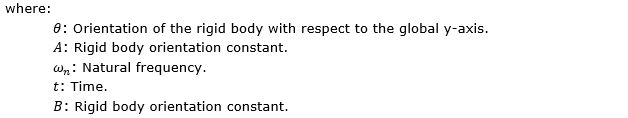
The solution to the equation of motion for a rotating rigid body subjected to undamped free vibration is expressed as follows:
Recall that Equations 2 and 3 represents the angular velocity (
Using the known initial orientation ( Expression for the B constant using the initial rigid body orientation
Expression for the A constant using the initial angular velocity of a rigid body
Back-substituting equations 5 and 8 into equation 1, the angular motion of a rigid body subjected to undamped free vibration with a small angular displacement can be expressed in terms of the initial conditions, as follows:
Example 1:
Using Python for modeling the motion of a sphere fixed to a rotating rod subjected to undamped free vibration.
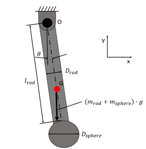
Create a plot that represents the motion of a sphere with a diameter of 25 mm with respect to time for 5 cycles (the time ranges from zero to five times the period of oscillation), where the sphere is fixed to the tip of a rod that is subjected to an undamped free vibration. The motion and the free-body diagram are depicted in figure 1. The rod diameter is 10 mm. The density of the rod and sphere materials is 0.00271 kg/mm3. Regardless of the rod lengths, the sphere is initially released at rest from θ = -10 deg. There should be 5 plots that depicts the motion of a sphere in the y-direction with respect to time, considering the rod lengths of 150 mm, 175 mm, 200 mm, 225 mm, and 250 mm. The plot should represent the position of the sphere center with respect to the pivot point in y-direction for different rod lengths. Additionally, create a plot that models the coordinates of the sphere center (relative to the pivot point) for the rod lengths of 150 mm, 175 mm, 200 mm, 225 mm, and 250 mm. At the end, there should be 10 plots in total.
< Figure 1: Pendulum motion subjected to an undamped free vibration. >
Mathematical Modelling:
Step 1: Analysis of mass and inertial properties. Mass of the rod and sphere
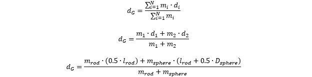
Position of center of pendulum mass with respect to the pivot point (i.e., point O from figure 3)
Rotational moment of inertia at the pivot point
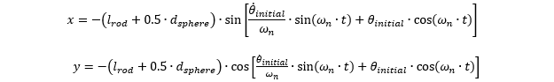
Step 2: Equation of motion for the sphere center with respect to the pivot point. Equation of motion in the x and y directions
Equation of the angular motion
The natural frequency of the rod and the sphere is,
Combining the equations of motion,
The period of motion is:
Python Code:
import numpy as np import matplotlib.pyplot as plt
# Inputs # d_sphere : Sphere diameter [mm]. # d_rod : Rod diameter [mm]. # l_rod : Rod length [mm]. # rho : Material density [kg/mm^3]. # theta_i : Initial input angle [rad]. # theta_dot_i : Initial angular velocity input [rad/s].
# Output # y : Position of the sphere center in the y-direction wrt to the pivot point [mm].
# Define the inputs num_t = 500 # number of time data. d_sphere = 25 d_rod = 10 rod_lengths = [150,175,200,225,250] n = len(rod_lengths) # number of elements in the rod_lengths array. # Create the array of rod lengths. The result should be the following: # l_rod = [[rod_lengths[0], rod_lengths[0], ... rod_lengths[0]], # [rod_lengths[1], rod_lengths[1], ... rod_lengths[1]], # . # . # . # [rod_lengths[n], rod_lengths[n], ... rod_lengths[n]]]
l_rod = np.zeros((n,num_t)) # n x num_t array initialization. for i in range(n): l_rod[i,:] = rod_lengths[i] rho = 0.00271 theta_i = -10*np.pi/180 theta_dot_i = 0.0
# Analysis of mass and inertial properties. # The columns should be identical for all the initialized arrays below. # The rows are dependent on the rod lengths. m_sphere = rho*np.pi*d_sphere**2/3 # mass of the sphere m_rod = np.zeros((len(l_rod),num_t)) # mass of the rod d_G,I_O = np.zeros((len(l_rod),num_t)),np.zeros((len(l_rod),num_t)) # center of mass to pivot point distance, rotational moment of inertia at the pivot point
for i in range(len(l_rod)): m_rod[i,:] = rho*np.pi*d_rod**2*l_rod[i]/4 d_G[i,:] = (m_rod[i]*0.5*l_rod[i] + m_sphere*(l_rod[i] + 0.5*d_sphere))/(m_rod[i] + m_sphere) I_O[i,:] = 1/12*m_rod[i]*l_rod[i]**2 + 1/10*m_sphere*d_sphere**2 + (m_rod[i] + m_sphere)*d_G[i]**2
# Natural frequency and period of oscillation analysis g = 9810 # mm/s^2 # The columns should be identical for all the initialized arrays below. # The rows are dependent on the rod lengths. omega_n,T = np.zeros((len(l_rod),num_t)),np.zeros((len(l_rod),num_t)) # natural frequency, period of oscillation
for i in range(len(l_rod)): omega_n[i,:] = np.sqrt((m_rod[i,:] + m_sphere)*g*d_G[i,:]/I_O[i,:]) T[i,:] = 2*np.pi/omega_n[i,:]
# Create a for-loop algorithm to create the arrays that contain the time inputs # for different rod lengths. The rows are dependent on the rod lengths. t = np.zeros((len(l_rod), num_t)) for i in range(len(l_rod)): t[i,:] = np.linspace(0.0,5.0*T[i][0],num=num_t)
theta = theta_dot_i/omega_n*np.sin(omega_n*t) + theta_i*np.cos(omega_n*t) y = -(l_rod + 0.5*d_sphere)*np.cos(theta)
# Create the plots to show the relationship between the pendulum motion in the y-direction and time. for k in range(len(l_rod)): plt.figure(k) plt.plot(t[k,:],y[k,:],'bo',t[k,:],y[k,:],'k') plt.xlabel('t [s]') plt.ylabel('y [mm]') plt.title('y vs t') plt.show()
# Create the plots to show the relationship between the pendulum motion in x and y directions from theta = theta_initial to theta = -theta_initial (theta_initial < 0). x = -(l_rod + 0.5*d_sphere)*np.sin(theta) for k in range(len(l_rod),2*len(l_rod)): plt.figure(k) plt.plot(x[k-len(l_rod),:],y[k-len(l_rod),:],'bo',x[k-len(l_rod),:],y[k-len(l_rod),:],'k') plt.xlabel('x [mm]') plt.ylabel('y [mm]') plt.title('y vs x') plt.show()
# Create the plots (in the same space) to show the relationship between the pendulum motion in the y-direction and time. plt.figure(1) plt.plot(t[0,:],y[0,:],'b.',t[0,:],y[0,:],'b', label='l_rod = 150 mm') plt.plot(t[1,:],y[1,:],'g.',t[1,:],y[1,:],'g', label='l_rod = 175 mm') plt.plot(t[2,:],y[2,:],'r.',t[2,:],y[2,:],'r', label='l_rod = 200 mm') plt.plot(t[3,:],y[3,:],'m.',t[3,:],y[3,:],'m', label='l_rod = 225 mm') plt.plot(t[4,:],y[4,:],'k.',t[4,:],y[4,:],'k', label='l_rod = 250 mm') plt.xlabel('t [s]') plt.ylabel('y [mm]') plt.title('y vs t') plt.legend() plt.show()
# Create the plots (in the same space) to show the relationship between the pendulum motion in x and y directions. x = -(l_rod + 0.5*d_sphere)*np.sin(theta) # Motion in x-direction. plt.figure(2) plt.plot(x[0,:],y[0,:],'b.',x[0,:],y[0,:],'b', label='l_rod = 150 mm') plt.plot(x[1,:],y[1,:],'g.',x[1,:],y[1,:],'g', label='l_rod = 175 mm') plt.plot(x[2,:],y[2,:],'r.',x[2,:],y[2,:],'r', label='l_rod = 200 mm') plt.plot(x[3,:],y[3,:],'m.',x[3,:],y[3,:],'m', label='l_rod = 225 mm') plt.plot(x[4,:],y[4,:],'k.',x[4,:],y[4,:],'k', label='l_rod = 250 mm') plt.xlabel('x [mm]') plt.ylabel('y [mm]') plt.title('y vs x') plt.legend() plt.show()
# Create the plots to show the relationship between the pendulum orientation and time. plt.figure(3) plt.plot(t[0,:],theta[0,:],'b.',t[0,:],theta[0,:],'b', label='l_rod = 150 mm') plt.plot(t[1,:],theta[1,:],'g.',t[1,:],theta[1,:],'g', label='l_rod = 175 mm') plt.plot(t[2,:],theta[2,:],'r.',t[2,:],theta[2,:],'r', label='l_rod = 200 mm') plt.plot(t[3,:],theta[3,:],'m.',t[3,:],theta[3,:],'m', label='l_rod = 225 mm') plt.plot(t[4,:],theta[4,:],'k.',t[4,:],theta[4,:],'k', label='l_rod = 250 mm') plt.xlabel('t [s]') plt.ylabel('theta [rad]') plt.title('theta vs t') plt.legend() plt.show()
Python Results:
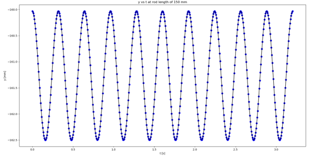
< Figure 2: Pendulum motion in the y-direction with respect to time at the rod length of 150 mm >
The x-axis represents time and y-axis represents the pendulum motion in the y-direction.
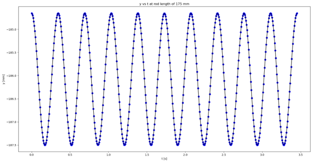
< Figure 3: Pendulum motion in the y-direction with respect to time at the rod length of 175 mm >
The x-axis represents time and y-axis represents the pendulum motion in the y-direction.
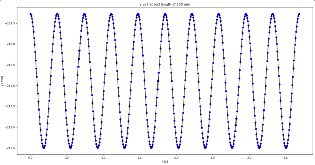
< Figure 4: Pendulum motion in the y-direction with respect to time at the rod length of 200 mm. >
The x-axis represents time and y-axis represents the pendulum motion in the y-direction.
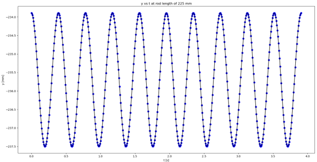
< Figure 5: Pendulum motion in the y-direction with respect to time at the rod length of 225 mm. >
The x-axis represents time and y-axis represents the pendulum motion in the y-direction.
< Figure 6: Pendulum motion in the y-direction with respect to time at the rod length of 225 mm. >
The x-axis represents time and y-axis represents the pendulum motion in the y-direction
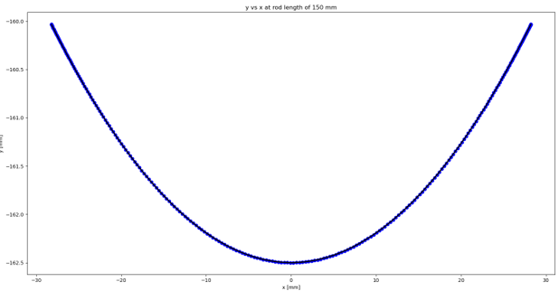
< Figure 7: Sphere center coordinates at the first-half of a cyclic motion at the rod length of 150 mm >
The x and y axes represent the x and y coordinates, respectively.
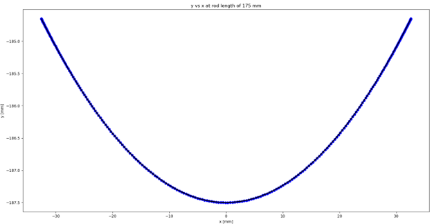
< Figure 8: Sphere center coordinates at the first-half of a cyclic motion at the rod length of 175 mm >
The x and y axes represent the x and y coordinates, respectively.
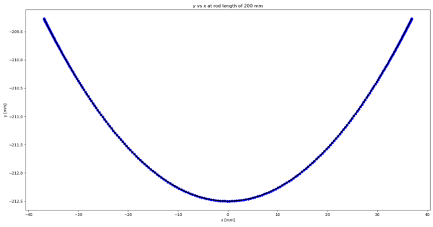
< Figure 9: Sphere center coordinates at the first-half of a cyclic motion at the rod length of 200 mm. >
The x and y axes represent the x and y coordinates, respectively.
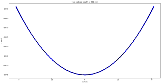
< Figure 10: Sphere center coordinates at the first-half of a cyclic motion at the rod length of 225 mm. >
The x and y axes represent the x and y coordinates, respectively.
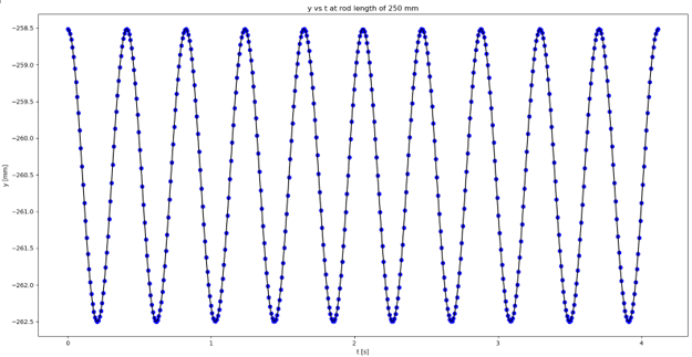
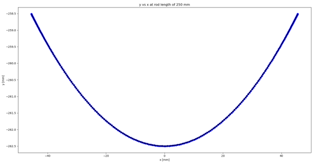
< Figure 11: Sphere center coordinates at the first-half of a cyclic motion at the rod length of 250 mm >
The x and y axes represent the x and y coordinates, respectively.
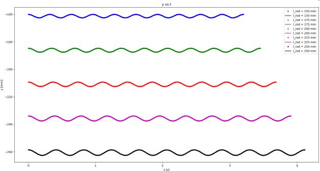
< Figure 12: Pendulum motion in the y-direction with respect to time at different rod lengths. >
The x-axis represents time and y-axis represents the pendulum motion in the y-direction.
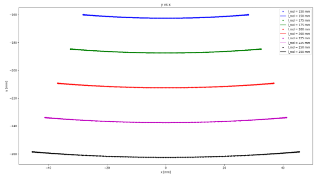
< Figure 13: Sphere center coordinates at the first-half of a cyclic motion at different rod lengths.>
The x and y axes represent the x and y coordinates, respectively.
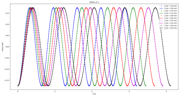
< Figure 14: Angular motion of the pendulum with respect to time at different rod lengths. >
The x-axis represents the pendulum orientation and y-axis represents the pendulum motion in the y-direction.
Insights on figures 12 to 14: The increase in rod lengths translate to an increase in both the period of oscillation (and in turn a decrease in oscillation frequency) and the amplitude of the cosine waves. The increase in amplitude indicates a higher displacement of the sphere in the vertical direction from θ = -10 deg to θ = 0 deg. Additionally, the increase in rod lengths also translate to an increase in displacement of the sphere in the horizontal direction from θ = -10 deg to θ = 10 deg. As shown in figure 14, the angular displacement (i.e., min. theta to max. theta) is not affected by the rod length. However, the increase in rod length translates to an increase in the period of oscillation, and in turn a decrease in frequency.
Reference :
|
||