|
Duffing Oscillator
Duffing oscillator is a classic example used to demonstrate chaotic behavior and dynamics. It is represented in mathematical form as follows (the details of the form and symbols may vary depending on the documents, but overall form would be similar to this).
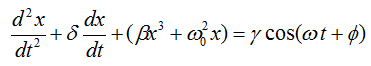
The meaning of each terms and coefficients are as follows :
x = displacement
x' = velocity
x'' = acceleration
δ = damping coefficient
ω0 = natural frequency of oscillation
β = nonlinearity coefficient
γ = forcing amplitude
ω = forcing frequency
φ = phase shift of forcing function
The characteristics of this equation can be summarized as follows :
- The x3 term introduces nonlinearity which enables chaotic dynamics.
- The system exhibits chaotic, bounded oscillations for certain parameter ranges.
- Varying the forcing frequency ω relative to the natural frequency ω0 impacts the behavior.
- The oscillations switch between periodic and chaotic as parameters change.
- Slight changes in initial conditions yield dramatically different trajectories over time.
- The phase shift φ of the external forcing alters when chaotic regimes emerge.
- Tools like phase portraits and Poincar� sections reveal the underlying attractor.
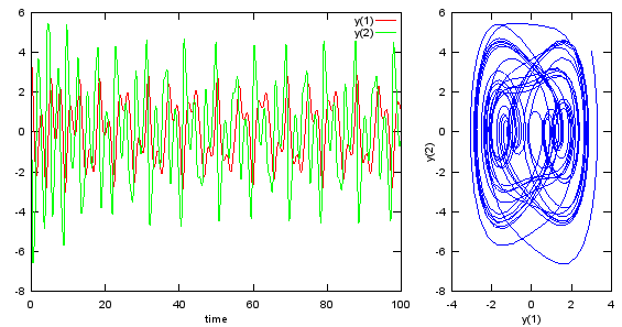
You can plot out the solution of this equation using a simple script below. Play with parameters and initial conditions and see how the plot changes.
| Matlab |
%Save the following contents in a .m file and run the .m file
% this is tested only in Matlab, not in Octave
delta = 0.06;
beta = 1.0;
w0 = 1.0;
w = 1.0;
gamma = 6.0;
phi = 0;
dy_dt = @(t,y) [y(2);...
-delta*y(2)-(beta*y(1)^3 + w0^2*y(1))+gamma*cos(w*t+phi)];
odeopt = odeset ('RelTol', 0.00001, 'AbsTol', 0.00001,'InitialStep',0.5,'MaxStep',0.5);
[t,y] = ode45(dy_dt,[0 100], [3.0 4.1],odeopt);
subplot(1,3,[1 2]);plot(t,y(:,1),'r-',t,y(:,2),'g-'); xlabel('time'); legend('y(1)','y(2)');
subplot(1,3,3);plot(y(:,1),y(:,2)); xlabel('y(1)'); ylabel('y(2)');
|
| Python |
# make it sure that you installed all these packages
import numpy as np
from scipy.integrate import odeint
import matplotlib.pyplot as plt
# Parameters
delta = 0.06
beta = 1.0
w0 = 1.0
w = 1.0
gamma = 6.0
phi = 0
# Derivatives function
def duffing(y, t):
y1, y2 = y
dydt = [y2,
-delta*y2 - beta*y1**3 + w0**2*y1 + gamma*np.cos(w*t + phi)]
return dydt
# Initial conditions
y0 = [3.0, 4.1]
# Integrate
t = np.linspace(0, 100, 3000)
sol = odeint(duffing, y0, t)
# Plot
fig = plt.figure(figsize=(12, 4))
ax1 = plt.subplot2grid((1, 3), (0, 0), colspan=2)
ax1.plot(t, sol[:,0], 'r-', t, sol[:,1], 'g-')
ax1.set_xlabel('Time')
ax1.legend(['y(1)','y(2)'])
ax2 = plt.subplot2grid((1, 3), (0, 2))
ax2.plot(sol[:,0], sol[:,1])
ax2.set_xlabel('y(1)')
ax2.set_ylabel('y(2)')
plt.tight_layout()
plt.show()
|
|
|