GF(2) is the smallest useful number system in communication engineering, and it has only two members. That sounds like a curiosity until you notice that every CRC, every convolutional code and every LDPC parity check is arithmetic in this field. This page gives the rules first and then works four examples through by hand.

• What is GF(2) ?
• How do addition and multiplication work ?
• How is a binary number written as a polynomial ?
• Examples :
• Example 1 : Addition of GF(2) Polynomial
• Example 2 : Multiplication of GF(2) Polynomial
• Example 3 : Division of GF(2) Polynomial
• Example 4 : Application of GF(2) - CRC Checksum Bit Calculation

What is GF(2) ?

Galois Field is a term that is made up of 'Galois' (name of a person) and 'Field' (a mathematical term).  Galois Field is a kind of Field that is contains a finite number of elements. Explaining about 'What is Field' is not a scope of this page. To be honest, I don't have enough mathematical knowledge to describe the concept of Field in my own words.

Even so, a short working definition helps, and it needs very little mathematics. Let's take the two words one at a time.

A field is a set of values with two operations defined on it, addition and multiplication. Subtraction and division are not separate requirements. Subtraction means adding the additive inverse, and division means multiplying by the multiplicative inverse. So a field has only two things to guarantee. Every element needs an additive inverse, and every element except 0 needs a multiplicative inverse. Once both hold, all four operations work and every answer stays inside the set.

That last sentence is worth checking rather than believing, because {0, 1} looks far too small to survive a subtraction. It survives because both inverses are already in the set. The additive inverse of 1 is 1, since 1 + 1 = 0, which is the line Figure 2 draws out as 1 = -1. The multiplicative inverse of 1 is 1, since 1 x 1 = 1. Zero needs no multiplicative inverse, and no field gives it one.

So the four operations can be written out in full, and the table below does that. Every entry is 0 or 1. The only blank is division by zero, which is undefined in every field, including the rational numbers.

Read the a - b column next to the a + b column and they are identical. That is the whole content of 1 = -1: in GF(2) subtracting is the same operation as adding, so one XOR gate does both. The a / b column is shorter still, because the only value you are ever allowed to divide by is 1, and dividing by 1 changes nothing.

The trap here is doing the arithmetic over the ordinary integers. There 0 - 1 is -1, which is not in the set, and the closure claim looks false. In GF(2) every result is reduced mod 2, and -1 mod 2 is 1. The set is closed once you use the field's own arithmetic rather than integer arithmetic.

Familiar examples make the test concrete. The rational numbers form a field, and so do the real numbers. The whole numbers do not, because 1 divided by 2 is not a whole number. That is a stricter test than it first looks, and most sets of numbers fail it.

Finite is the other word, and it means the set holds a fixed number of members and no more. You cannot keep counting upward. When an operation would carry a result past the end of the list, the value wraps around to the start, so the answer stays inside the set.

A clock face is the everyday version of that wrapping. Nine o'clock plus five hours is two o'clock rather than fourteen, because the positions stop at twelve and begin again. The analogy is close but not exact. On a clock 3 times 4 reaches 12, and 12 sits at the same position as 0, so no number multiplies 3 back to 1. Division breaks there, and a set where division breaks is not a field.

That failure explains a rule worth knowing. A finite field exists only when the number of elements is a prime number, or a power of a prime. Twelve is neither, which is why the clock fails the test. Two is prime, so GF(2) works, and it is the smallest finite field there is.

The number in the brackets is simply the count of elements. GF(2) has two, GF(4) has four, and GF(256) has 256, which is the field behind Reed-Solomon codes and AES. The name honours Evariste Galois, the French mathematician who established which of these systems can exist at all.

GF(2) represents a kind of Galois Field that is made up of only two elements 0 and 1. It can be represented in mathematical term as follows.

Figure 1. GF(2) is the two element set {0, 1}. The note on the right says the same thing twice: once as a set, and once as the coefficients a polynomial over this field is allowed to take.

Another way to see the same field is as ordinary integer arithmetic with only the remainder after division by 2 kept. That is what the Z/2 in Figure 1 means. Add 1 and 1, get 2, keep the remainder 0. This view is the one that explains every mod 2 step in the worked examples further down.

The reason engineers care is that the field is finite. A finite field has no rounding, no overflow and no approximation, so a calculation gives the same exact answer on any machine and in any order. That is precisely what an error detecting code needs, because the transmitter and the receiver have to agree bit for bit.

You can think of GF(2) as a special mathematical tools that explains various properties of binary operation (mathematical operations about binary numbers). The reason why this is important in communication is that the digital communication is based on binary data and various mathematical operations dealing with binary numbers. You wouldn't see this term on every day job in communication engineering, but many technologies (especially 'coding' techniques) are based on this theory even though you are not aware of it.

• A field is a set where all four operations stay inside it : add, subtract, multiply or divide two members and the answer is still a member. Only division by zero is excluded.
• Only addition and multiplication are axioms : subtraction and division follow from the inverses, which is why checking GF(2) takes only the two tables in Figure 2 and Figure 3.
• Finite means the values wrap rather than run on : the set has a fixed size, so an operation that would overshoot the end comes back to the start instead.
• The element count must be a prime or a power of one : that is why GF(2), GF(4) and GF(256) exist and a twelve position clock is not a field.
• GF(2) is the smallest field that exists : two elements is the least a field can have. Those two are exactly the 0 and 1 a digital system already works in.

How do addition and multiplication work ?

Two operations are all a field needs, and in GF(2) both of them fit in a four line table. The tables below are worth memorising rather than looking up, because everything later on this page is these two rules applied over and over.

Some important rules (properties) of GF(2) can be summarized as follows. Simply put, the two most common operation is GF(2) is 'Addition' and 'Multiplication'. These two operations are defined as follows.

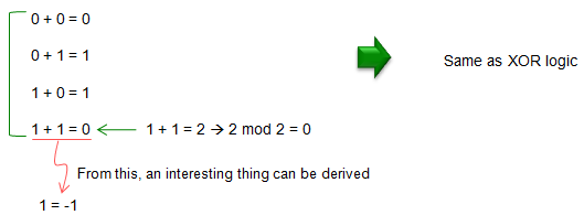
Figure 2. Addition in GF(2). 1 + 1 gives 2, and 2 mod 2 is 0, so the table is exactly XOR. The line underneath draws the consequence: 1 = -1, which makes subtraction and addition the same operation.

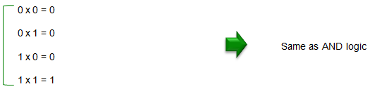
Figure 3. Multiplication in GF(2), which is exactly AND. Between them, Figure 2 and this table are the entire arithmetic of the field.

Those two tables are worth more attention than their size suggests. Addition is XOR, multiplication is AND, and there is nothing else to learn. A processor already has both gates, so arithmetic in this field costs one gate delay rather than an adder.

The note under Figure 2 is the part that surprises people. If 1 + 1 = 0, then 1 is its own negative, and subtracting is the same as adding. So GF(2) arithmetic has no carry, no borrow and no sign. Every column of a calculation is independent of every other column, which is why the hardware is a row of XOR gates and why the order you process the bits in does not matter.

Those two tables are the complete arithmetic of GF(2), and it is worth being clear about why nothing else is needed. A field is defined by addition and multiplication alone. The subtraction and division columns in the closure table were not extra rules, because each one was read off these two tables by way of an inverse. So once you can fill in these eight lines, you can answer any arithmetic question the field can pose.

• Addition is XOR and multiplication is AND : that is the whole field. Anything else you meet in GF(2) is built from these two operations.
• There is no carry and no borrow : each column resolves on its own, so a calculation that would need a ripple carry in ordinary arithmetic finishes in one gate delay here.
• Adding and subtracting are the same thing : a long division over GF(2) therefore shows a plus sign where ordinary long division would show a minus. Figure 12 onwards uses exactly that convention.

How is a binary number written as a polynomial ?

The arithmetic above works on single bits, and real data arrives as a string of them. The bridge between the two is to read a bit string as a polynomial, and that one convention is what lets a whole block of data be divided in a single operation.

In most applications of GF(2), we represents a binary data into polynomials (Galois polynomials) and do various operations on those polynomials.  Rather than explaining too much, just going throug several examples would be more helpful.

The rule itself takes one line. Bit i becomes the coefficient of Xⁱ, counting from the right, so the rightmost bit is the constant term and the leftmost bit is the highest power. The bit string 1011 therefore reads as 1X³ + 0X² + 1X + 1, which is written X³ + X + 1. Reading a polynomial back as bits runs the same rule in reverse.

One point is easy to get wrong. X is a placeholder for a bit position and never a number you substitute. Nobody evaluates X³ + X + 1 at X = 2. The polynomial is a way of naming which bit positions hold a 1, and the powers of X are there to keep the positions from mixing during a calculation.

So why convert to polynomials at all, when the bits were perfectly readable already? Because polynomials bring an operation that bit strings do not have on their own, which is division with a remainder. Dividing one polynomial by another always leaves a remainder whose degree is smaller than the divisor's, so the remainder has a known and fixed length. That is exactly the guarantee a CRC needs, and Example 4 is where it is used.

Degree is the other thing the notation makes obvious. The degree of a polynomial is the position of its highest set bit, so a degree 5 generator produces a remainder of degree 4 or less, which is 5 bits. So you can read the number of CRC bits straight off the generator polynomial.

• Bit i is the coefficient of Xⁱ : the conversion is a relabelling and no arithmetic happens in it. 1011 and X³ + X + 1 are two spellings of the same thing.
• X is never evaluated : it marks a bit position. Trying to substitute a value for it is the single most common misreading of this notation.
• The point of the detour is division : polynomials come with a remainder of bounded degree, and that bound is what makes a fixed length checksum possible.
• The generator's degree sets the CRC length : a degree 24 generator gives 24 CRC bits. That is why LTE names its polynomials CRC24, CRC16 and CRC8.

Examples :

Addition and multiplication below use the same pair of polynomials, so you can compare the two operations directly. Division uses a different pair, and the CRC example then reuses the division example exactly. That repeat is the quickest way to see that a CRC is nothing more than a remainder.

Example 1 : Addition of GF(2) Polynomial

Addition is the operation to start with, because it is the one that turns out to be a single machine instruction. Watch the middle step in particular: writing the zero coefficients in is what makes the rest of the calculation mechanical.

Figure 4. The two polynomials to be added, written the ordinary way with the zero terms left out.

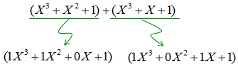
Figure 5. The same pair with every coefficient written in, zeros included. Lining the terms up by power is what makes the next step mechanical.

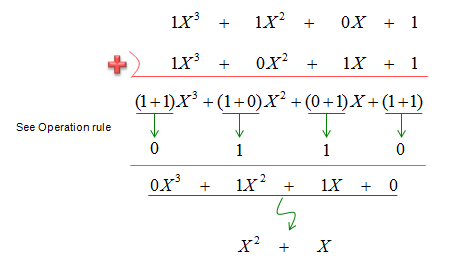
Figure 6. Adding coefficient by coefficient. The X³ column and the constant column both give 1 + 1, which is 0, so both terms disappear and the answer is X² + X.

Notice what the middle step achieves. Writing out 1X³ + 1X² + 0X + 1 instead of X³ + X² + 1 costs one line. It removes all the bookkeeping, because every power then has a column and no term can be skipped by accident.

There is a shortcut worth knowing, and it is the reason this example matters. Write each polynomial as its coefficient string: X³ + X² + 1 becomes 1101 and X³ + X + 1 becomes 1011. XOR the two strings and you get 0110, which reads back as X² + X. That is the same answer the long form produced. Polynomial addition over GF(2) is a bitwise XOR of the coefficient strings, and nothing more.

• Write the zero terms in : the step that looks like padding is the step that makes the addition mechanical, because every power gets its own column.
• A term survives only if it appears once : a power present in both polynomials cancels, and a power present in neither stays absent. Only the powers in exactly one of them reach the answer.
• In bits it is one XOR : 1101 XOR 1011 = 0110. A processor does this whole example in a single instruction.

Example 2 : Multiplication of GF(2) Polynomial

Multiplication uses the same two polynomials the addition example used, so anything different in the answer comes from the operation rather than from the inputs. Watch for the one column where a coefficient comes out larger than 1, because that is the only place the field rule is needed.

Figure 7. The two polynomials to be multiplied. They are the same pair the addition example used, so any difference in the answer comes from the operation rather than from the inputs.

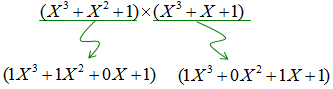
Figure 8. The same pair with all coefficients written in, ready to be multiplied term by term.

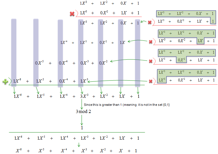
Figure 9. The four partial products, summed column by column. One column needs the field rule. X³ collects a coefficient of 3, and 3 mod 2 is 1, so the answer is X⁶ + X⁵ + X⁴ + X³ + X² + X + 1.

The multiplication itself is ordinary long multiplication. Each term of one polynomial multiplies the whole of the other, the partial products are shifted so that equal powers line up, and the columns are added. Nothing in that description belongs to GF(2).

The field rule applies once, at the end. A coefficient of 3 is not a member of {0, 1}, so it is reduced mod 2 and becomes 1. That single reduction is the only place this calculation differs from the one you would do over ordinary integers. The note beside it says as much, by pointing out that 3 is not in the set.

Multiplication does not have the neat bitwise shortcut that addition has. Shifting and XOR-ing gets you the partial products, but you still have to accumulate them, so a multiply costs far more than an add. That asymmetry is the reason CRC hardware is built around division and addition rather than around multiplication.

• Multiply as usual, then reduce mod 2 : the long multiplication is the familiar one. GF(2) only decides what to do with a coefficient that comes out bigger than 1.
• Only one column needed the rule here : the X³ column collected three contributions. Every other column collected 0 or 1 and needed nothing doing to it.
• Multiplication is the expensive operation : addition is a single XOR and multiplication is a shift-and-accumulate loop, which is why practical coding schemes lean on addition and division.

Example 3 : Division of GF(2) Polynomial

Division is the operation that CRC actually uses, and it is worth following slowly. The six pictures below build the quotient one term at a time. Each one repeats everything above it with a single line added, so read them as one calculation rather than as six.

NOTE : In this process, you see the following operations. This two step operation is same as 'XOR' in binary number. In real compuation (especially in digital process, 'XOR' is used in stead of this kind of two step process).

Step 1 : Add coefficient values for each term

Step 2 : If the added value is less then 2 (i.e, 0 or 1), write the number as it is. If the added value is 2, apply 'mod 2' to the numbr (i.e, if the value is 2, change the number to 0).

Figure 10. The division to be performed, written in the ordinary compact form.

Figure 11. Dividend and divisor with every coefficient written in. The divisor has degree 5, so the remainder will end up with degree 4 or less.

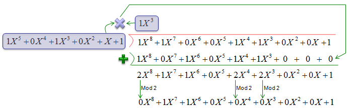
Figure 12. The first step. X³ times the divisor is added, which in GF(2) is the same as subtracting it, and each coefficient that comes out as 2 is reduced to 0. The leading term cancels, which is the whole point of choosing X³.

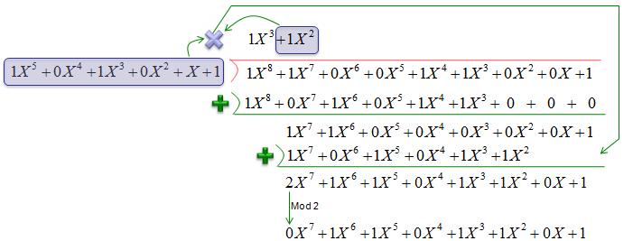
Figure 13. The second step adds X² to the quotient and cancels the new leading term.

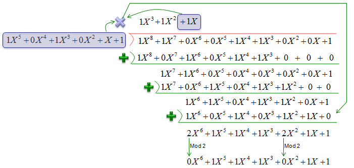
Figure 14. The third step adds X to the quotient.

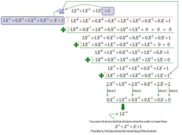
Figure 15. The fourth step adds 1 to the quotient. What is left is X⁴, whose degree is below the divisor's, so the division stops. The quotient is X³ + X² + X + 1 and the remainder is X⁴.

The loop is the same one you learned for ordinary long division. Look at the leading term of what is left, choose the quotient term that will cancel it, multiply the divisor by that term, add the result, and repeat. The division ends when the degree of what remains falls below the degree of the divisor.

Two things make the GF(2) version easier rather than harder. There is no carry, so each column reduces on its own. And the quotient term is always either 0 or 1, so there is no trial and error about how many times the divisor goes in. You compare the leading degrees and the answer is immediate.

You can check the result without redoing the work. Multiply the quotient by the divisor and add the remainder, and you should recover the dividend. Doing that here gives X⁸ + X⁷ + X³ + 1 from the product. Add the remainder X⁴ and you get back X⁸ + X⁷ + X⁴ + X³ + 1, which is the dividend the example started from.

• The quotient digit is never in doubt : it is 1 when the leading degrees match and 0 when they do not. Ordinary long division has to guess and check; this one does not.
• The remainder is what the division is really for : the quotient is discarded in almost every application. CRC keeps the remainder and throws the quotient away.
• Check by multiplying back : quotient times divisor plus remainder has to return the dividend. It is a two minute check and it catches a dropped column immediately.

Example 4 : Application of GF(2) - CRC Checksum Bit Calculation

Nothing in this example is new arithmetic. It is the division from Example 3 with the parts renamed, which is the quickest way to see what a CRC actually is once you set the vocabulary aside.

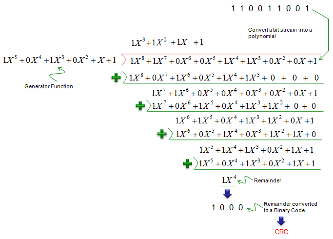
Figure 16. The same division again, labelled this time as a CRC calculation. The dividend, the generator, the quotient and the remainder are all the ones from Example 3, and the remainder written back as bits is the CRC.

Read Figure 16 next to Figure 15 and the point of the whole page becomes clear. The arithmetic has not changed at all. What changed is the vocabulary: the divisor is now called the generator function, the dividend is a block of data rather than an abstract polynomial, and the remainder has a name, CRC.

The translation at each end is the only new material. A bit stream becomes a polynomial by making bit i the coefficient of Xⁱ, which is the step the arrow at the top of the picture marks. At the other end the remainder becomes a bit pattern the same way, and those are the bits the transmitter appends to the data.

So a CRC is a remainder, and that is the whole of it. The receiver runs the same division over the data with the CRC attached, and a remainder of zero means no error was detected. Everything else in a CRC specification is a choice of generator polynomial, which decides which error patterns the remainder will catch.

• A CRC is the remainder of a GF(2) division : nothing in Example 4 is new arithmetic. It is Example 3 with the parts renamed.
• The generator polynomial is the only design choice : its degree fixes the number of CRC bits, and its particular terms decide which error patterns cannot slip through.
• Bit stream to polynomial and back is just relabelling : bit i is the coefficient of Xⁱ in both directions. No arithmetic happens in the conversion.